Bank statement velocity — the rate, frequency, and directional trend of deposits and transactions over time — is one of the strongest predictors of working capital loan repayment success. Underwriters who track five core velocity metrics across a 3-to-6-month window can identify repayment risk signals weeks before traditional cash flow analysis surfaces any warning.
What you'll learn
- Bank statement velocity measures the rhythm of cash flow over time, making it a leading indicator of repayment capacity rather than a lagging one
- Five velocity metrics — DFR, GDVT, NDV, ADBD, and BRR — form a practitioner framework for predicting working capital loan repayment outcomes
- Declining velocity in the final 30 days of a bank statement window is the single most important early warning signal for near-term default risk
- MCA stacking produces a distinct velocity signature — rising ACH debit-to-deposit ratios and net deposit velocity compression — detectable before credit checks
- Automated bank statement parsing enables velocity analysis at scale across 900+ bank formats, making portfolio-level velocity benchmarking operationally viable
Bank statement velocity — the rate, frequency, and directional trend of deposits and transactions over time — is one of the strongest predictors of working capital loan repayment success. Underwriters who track five core velocity metrics across a 3-to-6-month window can identify repayment risk signals weeks before traditional cash flow analysis surfaces any warning.
What Is Bank Statement Velocity — And Why Most Underwriters Underuse It
Bank statement velocity is a discrete, measurable underwriting concept: the rate, frequency, and directional trend of deposit and transaction activity over a defined time window. It's not a single number. It's a dynamic portrait of how a business generates and cycles cash — and whether that behavior is accelerating, holding steady, or breaking down.
Most underwriting frameworks don't treat velocity this way. They treat bank statements as a source of static inputs: gross monthly deposits, average daily balance, NSF count. These are snapshot metrics. They tell you what happened on average. They don't tell you whether things are getting better or worse right now.
According to FDIC data on small business lending, cash flow volatility — not credit score — is the primary driver of short-term loan default among businesses with fewer than 500 employees. Yet most underwriting checklists still anchor risk assessment to backward-looking averages. Velocity fills the gap by revealing directional changes in business activity in near real time.
When building out your broader underwriting process, velocity integrates naturally alongside other criteria in a complete MCA underwriting checklist — but it deserves its own analytical layer, not just a checkbox.
Velocity vs. Volume: Understanding the Difference
High gross deposit volume does not equal healthy velocity. A business can deposit $150,000 per month and still carry significant repayment risk if those deposits arrive in two or three large, irregular transactions rather than consistent daily or weekly inflows.
Consider two businesses with identical $90,000 quarterly deposits. Business A deposits $3,000–$5,000 four to five times per week, every week. Business B deposits $30,000 once per month. Same gross volume. Dramatically different repayment risk profiles for a short-term working capital loan drawing weekly repayments from that account.
Velocity captures the rhythm of cash flow, not just its magnitude. That rhythm is what determines whether there's money in the account when a repayment draws.
Why Traditional Cash Flow Metrics Miss the Signal
Average daily balance, net cash flow, and debt service coverage ratio (DSCR) are all backward-looking. They aggregate behavior across the full statement period and produce a single representative number. That number obscures what's happening in the most recent 30 days.
A business with strong average daily balance across a 3-month statement period can still be in active cash flow deterioration right now — if deposits slowed significantly in the final month. The average daily balance calculation won't surface that signal. Velocity does.
This is the core reason velocity is a leading indicator rather than a lagging one. It captures directional momentum — which is exactly what you need to predict near-term repayment performance.
The 5 Velocity Metrics That Predict Working Capital Loan Repayment
The following five metrics form a practitioner framework for working capital loan underwriting based on transaction velocity. Each metric is calculable from parsed bank statement data. Each has defined threshold ranges. No single metric is sufficient in isolation — the value is in reading them together.
1. Deposit Frequency Rate (DFR)
Deposit Frequency Rate measures the number of distinct deposit transactions per week, averaged across the statement period.
Calculation: Total deposit transaction count ÷ total weeks covered by the statement.
Threshold guidance:
- DFR below 2 per week over a 3-month window: elevated default risk. Deposits are too infrequent to reliably service weekly or daily repayment draws.
- DFR of 2–4 per week: moderate. Acceptable for longer repayment terms, warrants additional scrutiny for short-term products.
- DFR above 5 per week: consistent cash generation. Positive repayment capacity signal.
DFR matters more than deposit size for short-term repayment capacity. A business depositing every day at $1,000 is a safer MCA candidate than one depositing $10,000 twice per month — because repayment draws happen on the same cadence as deposits.
2. Gross Deposit Velocity Trend (GDVT)
Gross Deposit Velocity Trend measures the month-over-month percentage change in total gross deposit volume. It captures whether top-line business activity is growing, flat, or declining.
Calculation: ((Current month gross deposits − Prior month gross deposits) ÷ Prior month gross deposits) × 100.
GDVT is distinct from net cash flow velocity. Gross captures the top line — all incoming deposits regardless of what goes out. That's useful because it isolates revenue-side momentum from cost-side changes.
- Two consecutive months of declining GDVT: yellow flag. Could be seasonal or temporary.
- Three consecutive months of declining GDVT: red flag. Structural revenue deterioration is the likely cause.
3. Net Deposit Velocity (NDV)
Net Deposit Velocity adjusts gross deposits by subtracting recurring fixed outflows — rent, payroll, known existing loan payments — before calculating the velocity trend. This is a materially different and more accurate metric for assessing true repayment capacity.
Calculation: (Gross deposits − Recurring fixed outflows) ÷ Time period.
To calculate NDV accurately, you need to identify and exclude recurring outflows from the raw transaction feed. Look for same-dollar-amount debits occurring on the same day each month — these are almost always fixed obligations.
The critical pattern to watch for is NDV compression: when NDV shrinks even as gross deposits hold steady. This signals rising fixed cost burden — meaning more of each dollar coming in is already committed before the business has a chance to service new debt.
Understanding NDV connects directly to the broader question of bank statement-based risk scores — velocity metrics like NDV are increasingly central inputs to composite risk models.
4. Average Days Between Deposits (ADBD)
Average Days Between Deposits calculates the mean number of calendar days elapsed between successive deposit transactions across the statement period.
Calculation: Sum of all inter-deposit intervals (in days) ÷ (total deposit count − 1).
ADBD is particularly useful as a trend metric rather than a point-in-time number. When ADBD is lengthening over the statement window, it signals that deposit activity is becoming less frequent — a leading indicator of cash flow stress.
- ADBD increasing by more than 30% in the final month vs. the prior two-month average: material risk signal. Deposits are spacing out, which creates repayment coverage gaps.
ADBD also helps distinguish seasonal patterns from structural deterioration. A retailer with ADBD lengthening every January (post-holiday slowdown) shows a different risk profile than a business with ADBD lengthening steadily across all three months of the statement window.
5. Balance Recovery Rate (BRR)
Balance Recovery Rate measures how quickly the account balance returns to its rolling average after a significant outflow event — a large payment, payroll run, or ACH withdrawal.
BRR is especially predictive for MCA repayment because MCAs draw from the account daily or weekly. If the balance doesn't recover quickly between draws, the business is living on an ever-thinner liquidity cushion.
- Slow BRR: balance stays depressed 5 or more days after a large outflow. Indicates thin liquidity and insufficient deposit frequency to absorb recurring draws.
- Fast BRR: balance recovers within 1–2 days. Indicates strong, frequent revenue inflows and real repayment capacity.
Together, these five metrics form a velocity profile that no single traditional underwriting metric can replicate. Here's how deposit velocity trends look visually across a 3–6 month statement window:
Note how rising and declining trend lines map directly to DFR and GDVT shifts — the patterns that separate repayable borrowers from at-risk ones are visible in the data before any default event occurs.
How to Read Deposit Frequency Patterns in Bank Statements
Metric definitions are the foundation. Pattern recognition is where working capital loan underwriting becomes a skill. The same DFR number can mean different things depending on how the underlying deposit pattern is shaped.
There are three core deposit frequency archetypes:
- Consistent daily or weekly deposits: healthy cash generation pattern. Revenue inflows are regular, predictable, and well-matched to repayment cadence. Lowest risk for short-term products.
- Lumpy large deposits: moderate risk. Business generates meaningful revenue but in irregular intervals — perhaps due to project-based billing or net-30 invoice cycles. Repayment timing risk is higher.
- Infrequent large deposits: high risk for short-term loan repayment. The account may look healthy on gross volume, but the gaps between deposits create sustained windows where repayment draws would overdraw the account.
Understanding how to normalize these patterns for seasonal businesses is equally important. A retailer's December surge, a landscaper's spring spike — these should not distort the annual velocity baseline. For seasonal revenue patterns, always compare current-period velocity against the same period in the prior year, not against the prior month.
3-Month vs. 6-Month Analysis Windows: What Each Reveals
The choice of analysis window materially changes what you can see in the velocity data.
| Analysis Window | Primary Value | Best Use Case | Limitation |
|---|---|---|---|
| 3 months | Recent trajectory, current business momentum | Short-term working capital, MCA underwriting | Seasonal distortion not visible |
| 6 months | Seasonal normalization, structural patterns | Larger loans, longer terms, seasonal businesses | Less sensitive to recent deterioration |
| 12 months | Full cyclical behavior, year-over-year comparison | Annual facilities, seasonal adjustment baseline | Most recent signal is diluted by prior-year data |
Best practice: run both the 3-month and 6-month windows and compare them. Divergence between windows is itself a signal. If the 6-month velocity looks healthy but the 3-month is declining, you're likely seeing the early stages of a deterioration that hasn't yet moved the longer-window averages.
For MCA underwriting specifically, the 3-month window carries more predictive weight. The repayment term is short. What happens in the next 90 days is what matters — and the most recent 90 days is your best proxy for that.
Normalizing Velocity for Seasonal Businesses
Applying DFR or GDVT thresholds rigidly to a seasonal business without normalization will produce false positives. A landscape company with January deposits 60% below June deposits isn't in decline — it's doing what landscape companies do in January.
The normalization framework:
- If 12 months of statements are available, identify the same-month pattern from the prior year as the baseline.
- Calculate seasonal-adjusted velocity: compare current-period metrics against the same period from the prior year, not the prior month.
- Flag when the business shows no seasonal recovery in a period where the prior year showed a clear uptick — that's the signal worth escalating.
The key distinction is between a business that's down 30% in January (normal for their seasonality) versus one that's down 30% compared to last January (potential structural deterioration). Only the latter is a genuine velocity warning.
Declining Velocity: The Early Warning Signal Hiding in Plain Sight
If there's one finding in this framework that should change how your team reviews bank statements, it's this: declining velocity in the final 30 days of the statement window is the single most important early warning signal in working capital loan underwriting.
Businesses that default on short-term loans almost always show a measurable velocity decline in the 30–60 days before the default event. That signal appears in the most recent statement month — the one that's most diluted when you're calculating 3-month averages.
The reason this signal hides: underwriters reviewing totals or monthly averages across the full statement period won't see a terminal 30-day decline. The final month's data is numerically averaged with the prior two months, smoothing away exactly the signal you need to catch.
The 30-day terminal decline pattern has three concurrent indicators:
- Deposit frequency (DFR) drops in the final month
- Average days between deposits (ADBD) lengthens
- Balance recovery rate (BRR) slows
When all three move in the same direction in the final 30 days, that's not noise. That's a business in active cash flow deterioration.
The balance tracker visualization above makes this pattern tangible — watch how account balance levels and recovery patterns degrade across 30-day buckets during a terminal velocity decline, compared to the stable pattern of a healthy borrower.
How to Segment Bank Statements for Terminal Velocity Analysis
The practical methodology for detecting terminal decline is straightforward:
- Divide the 3-month statement into three discrete 30-day buckets: Month 1 (oldest), Month 2, Month 3 (most recent).
- Calculate DFR, GDVT, and BRR for each bucket independently — not as a rolling average.
- Compare Month 3 metrics against the Month 1–2 average. Any metric declining by more than 20% in Month 3 relative to that average is a flag.
- Two or more metrics declining simultaneously in Month 3 is a strong default risk indicator. Treat it as a red flag requiring underwriter review, not a yellow flag requiring additional documentation.
This segmentation approach turns a 3-month bank statement from a summary document into a forward-looking trend analysis. It takes more time manually — but with automated parsing, the bucketed output is returned with no additional work required.
The NSF and Overdraft Connection to Velocity Decline
NSF events and overdraft days aren't separate issues from velocity decline — they're concurrent symptoms of the same liquidity stress event. In most default pre-cursors, NSF clustering and velocity decline appear in the same 30-day window.
The threshold that matters: more than 5 overdraft days per month in the terminal period is a disqualifying pattern for most underwriting frameworks. But the combination is what makes it dangerous. Rising NSF frequency alongside declining deposit velocity doesn't add risk linearly — it compounds it. The business is simultaneously generating less cash and failing to cover existing obligations.
For a deeper analysis of how NSF fees and overdraft patterns interact with velocity signals as concurrent liquidity stress indicators, the threshold analysis there complements this framework directly.
NSF clustering plus velocity decline equals a liquidity crisis in progress — not a temporary cash flow blip. Underwriting those applications requires either meaningful additional security or a decline.
Velocity Red Flags: Patterns That Correlate With Default
The following red flags represent patterns that appear consistently in bank statements prior to default events on working capital loans. Each is specific and quantifiable. Each has an underlying mechanism — fraud, financial stress, or active manipulation — that explains why it signals risk.
Round-Dollar Deposits and Artificial Velocity Inflation
Organic business cash flow is irregular. Real revenue deposits reflect actual sales: $4,847.32, $11,203.00, $6,912.50. Repeated round-dollar deposits — $5,000, $10,000, $25,000 — appearing with unusual frequency are a signal of fabricated or manipulated bank statements.
The mechanism: fraudsters add synthetic deposit entries to inflate DFR and GDVT. The fingerprint is round-dollar clustering — multiple round-number deposits within the same statement period, often at regular intervals.
Cross-reference this pattern with PDF metadata analysis. Backdated or altered transaction records often show metadata timestamps inconsistent with the claimed transaction dates. If the metadata and the round-dollar pattern both appear, treat the statement as potentially fraudulent pending additional verification.
For a detailed breakdown of how round-dollar deposit clustering is detected in automated systems, the pattern detection methodology extends well beyond manual review capabilities.
MCA Stacking Signatures in Velocity Data
MCA stacking — where a business takes multiple concurrent MCA positions without disclosing existing obligations — has a distinct velocity signature. You can detect it from bank statement data alone, before credit checks or disclosure review.
The stacking signature appears as:
- Rising number and increasing frequency of ACH debit transactions across the statement months
- Net deposit velocity compression despite stable or rising gross deposits
- Shrinking balance recovery rate as multiple daily ACH pulls compete with incoming deposits
Detection method: Calculate the ACH debit-to-deposit ratio for each 30-day bucket. A ratio rising across Month 1, Month 2, and Month 3 is a stacking signal. When the ACH outflow count grows while the deposit count holds flat, multiple funders are drawing from the same pool of incoming cash.
For the full methodology on detecting MCA stacking from bank statements, including how to cross-reference known MCA funder ACH originator IDs in the transaction feed, the stacking detection framework provides a complete investigative protocol.
The stacking detection visualization above shows how recurring ACH debit patterns accumulate against incoming deposit velocity — the compression is visible in the data weeks before the business reaches a repayment crisis.
Sudden Volume Spikes: Manipulation or Windfall?
A large deposit spike in Month 3 — the most recent month — can artificially inflate trailing metrics and mask an underlying declining trend. Underwriters who look at 3-month totals without segmentation will see a healthy aggregate picture that conceals deteriorating momentum.
The question to answer: is this a legitimate windfall or a manipulation? Use transaction description analysis to distinguish:
- Legitimate windfalls: tax refunds, invoice settlements from named counterparties, seasonal uptick matching prior-year patterns. These are real cash events — include them but note they are non-recurring.
- Suspicious spikes: single large transactions from uncharacteristic counterparties, transfers from related entities, deposits with generic or missing descriptions. Treat as non-recurring and exclude from velocity calculations.
Best practice: always recalculate DFR, GDVT, and NDV both with and without outlier deposits. If the velocity picture changes materially when you remove a single transaction, the approval decision should not rest on that transaction being real and recurring.
Manual vs. Automated Velocity Analysis: Speed, Scale, and Accuracy
Manual velocity analysis is possible. For a single application, an experienced underwriter who knows what to look for can segment the statement, calculate the five metrics, and check for red flags. The honest time estimate: 45–90 minutes per application to do it properly.
That includes segmenting the statement into 30-day buckets, calculating DFR, GDVT, NDV, ADBD, and BRR for each bucket, identifying and excluding recurring outflows for NDV, and scanning for round-dollar clustering, ACH stacking signatures, and terminal decline patterns.
At 20 applications per day, manual velocity analysis consumes an entire underwriter. At 50 applications per day, it's operationally unsustainable for any team.
The Hidden Cost of Manual Velocity Review
The labor math is straightforward. At a fully loaded underwriter cost of $35–$50 per hour, proper manual velocity analysis adds $26–$75 per application in labor cost. That's before accounting for errors.
Manual calculation of running balances and deposit frequency counts introduces systematic errors. Spreadsheet work at high volume produces miscounts, missed transactions, and miscategorized ACH debits. The error rate compounds at scale.
More importantly: underwriters reviewing totals — which is what most manual workflows actually produce — miss terminal-period segmentation in a significant portion of cases. They're scanning statement summaries, not bucketed 30-day trend analysis. The signal hides in the segmentation, not the summary.
For a detailed breakdown of the cost of manual bank statement review across underwriting workflows, the full labor and error cost analysis supports the case for automation compellingly.
At 100+ applications per day, portfolio-level velocity benchmarking — understanding what healthy DFR looks like across your specific borrower segment — becomes completely impossible through manual means.
What Automated Parsing Surfaces That Manual Review Misses
Automated bank statement parsing tools process all five velocity metrics simultaneously, across the full statement period and all 30-day buckets, for every application in a batch. The difference isn't just speed — it's analytical depth that's simply not achievable manually.
Automated systems identify round-dollar clustering, ACH stacking signatures, and terminal velocity decline in milliseconds. They apply the same segmentation methodology to every statement, every time, without fatigue or inconsistency.
For working capital lenders evaluating cash flow underwriting software, the velocity analysis capability — specifically whether the tool segments statements into 30-day buckets and calculates bucketed trend metrics — is the feature that separates serious underwriting infrastructure from basic parsing tools.
See Velocity Analysis Automated — In Real Time
See how ClearStaq surfaces all five velocity metrics — automatically, across every bank format — in the time it takes to open a spreadsheet. Book a 20-minute demo.
How ClearStaq Calculates Velocity Signals Across 900+ Bank Formats
Velocity calculations are only as reliable as the parsing that produces them. If a tool accurately parses Chase statements but misreads regional bank formats, your velocity metrics will be inconsistent across your application mix — which means your thresholds will be wrong for a portion of your portfolio. 900+ bank format support isn't a feature footnote — it's the foundational requirement for consistent velocity calculation across a real lender's book.
ClearStaq extracts all five velocity metrics directly from parsed transaction data, applies 30-day bucket segmentation automatically, and returns structured velocity trend analysis without requiring any post-processing by the underwriting team.
The 27 fraud signals embedded in the ClearStaq analysis include velocity-specific anomaly detection: round-dollar deposit clustering, sudden volume spikes inconsistent with prior-period patterns, and ACH-to-deposit ratio escalation signals. These are returned as structured alert objects alongside the raw velocity metrics.
PDF metadata and transaction timestamp analysis runs in parallel — catching backdated or altered statements before they corrupt velocity calculations. A manipulated statement with artificially inflated Month 3 deposits would produce incorrect GDVT and DFR metrics; metadata analysis catches the alteration before those numbers enter the underwriting workflow.
Velocity Metrics in the ClearStaq API Output
The ClearStaq API returns velocity data in structured JSON, including the following fields:
deposit_frequency_rate— DFR per week by month bucketgross_deposit_velocity_trend— Month-over-month GDVT percentagenet_deposit_velocity— NDV after recurring outflow exclusionaverage_days_between_deposits— ADBD by month bucket with trend directionbalance_recovery_rate— BRR per drawdown event with average recovery days
Month-by-month bucketed analysis is returned automatically — no post-processing, no spreadsheet work, no manual segmentation. Velocity anomaly flags are returned as structured alert objects, ready to gate decision logic in your loan origination system (LOS) directly via API integration.
From 100 Applications to Portfolio Intelligence
Batch processing of 100+ simultaneous bank statements enables something manual analysis categorically cannot: portfolio-level velocity benchmarking. What does a healthy DFR look like across your specific borrower segment — your industry mix, your loan size range, your geography? Generic industry averages don't answer that question. Your own portfolio data does.
When velocity trend data is processed at batch scale, lenders can calibrate their thresholds to reflect what actually predicts repayment success in their book — not what a published benchmark suggests. That calibration compounds in accuracy over time as more performance data accumulates.
SOC2 compliant data handling ensures sensitive financial document processing meets regulatory standards at every stage — a non-negotiable requirement when processing bank statements at institutional scale.
Building a Velocity-Based Underwriting Framework
The following framework synthesizes the velocity metrics, pattern detection, and threshold guidance from this post into a step-by-step process that any underwriting team can implement. It works alongside — not instead of — existing credit criteria. Velocity is additive to FICO, time in business, and revenue thresholds. It adds the predictive signal those metrics don't carry.
Step 1: Data Collection — How Many Months and Which Accounts
Data requirements depend on loan size and term:
- Minimum: 3 months of the primary operating account. Sufficient for short-term working capital loans and MCA underwriting. Provides enough data to calculate all five velocity metrics and perform terminal-period segmentation.
- Recommended: 6 months for loans above $100,000 or facilities with terms longer than 12 months. Enables seasonal normalization and structural pattern analysis.
- Ideal: 12 months when available. Use for seasonal adjustment baselines — compare current-month velocity against the same month from the prior year.
Include all accounts where business deposits flow. A business that splits deposits across two operating accounts will show artificially low DFR in any single account. Velocity calculated on one account when business revenue flows through two will understate actual deposit frequency. Consolidated multi-account analysis is required for accurate velocity metrics.
This connects directly to the practice of cross-referencing bank statements with tax returns — a complete data collection protocol uses multiple verification inputs, not just the bank statement alone.
Step 2: Scoring and Decision Logic
Apply the five velocity metrics through a structured scoring rubric:
| Velocity Score | Criteria | Decision Guidance |
|---|---|---|
| Green | All five velocity metrics trending stable or positive; no red flags in terminal 30-day period | Proceed to standard credit decision; velocity supports approval |
| Yellow | One metric declining in Month 3, or one red flag present (but not disqualifying) | Underwriter judgment required; request additional documentation or explanation |
| Red | Two or more metrics declining in terminal period; or any single disqualifying pattern (MCA stacking, round-dollar clustering, terminal decline trifecta) | Decline or require substantial additional security; escalate for senior review |
Velocity score should be weighted alongside DSCR and ADB in the final credit decision matrix. Document velocity rationale in the credit memo. This creates an audit trail and, over time, allows your team to correlate velocity scores with actual repayment outcomes — the data that enables threshold calibration.
Step 3: Integrating Velocity Into Your Existing Workflow
Velocity analysis adds approximately 3–5 minutes to a manual underwriting review when the underwriter is familiar with the framework. With automated parsing, it adds near-zero incremental time — the metrics are returned in the same API response as the standard bank statement data.
The most operationally efficient deployment is as a pre-screening gate: run velocity analysis before full underwriting. Applications with Red velocity scores are eliminated early, freeing underwriters to apply judgment to the applications that pass the velocity gate.
For MCA underwriters specifically: velocity analysis is more predictive than FICO for short-term repayment outcomes. FICO measures historical credit behavior. Velocity measures current cash flow behavior. For a 6-month MCA repayment term, what the business is doing with its cash right now is more informative than what it did with credit 2 years ago.
Understanding true revenue vs. gross revenue completes the picture: net deposit velocity (after recurring outflows) is the right denominator for repayment capacity analysis, for exactly the same reason that true revenue is a more accurate MCA sizing metric than gross deposit volume.
FAQ: Bank Statement Velocity and Working Capital Loan Underwriting
What is velocity in bank statement underwriting?
Bank statement velocity refers to the rate, frequency, and directional trend of deposit and transaction activity over a defined time window — typically 30 to 180 days. Unlike static metrics such as average daily balance, velocity measures whether cash flow activity is accelerating, stable, or declining, making it a leading rather than lagging indicator of repayment capacity.
How many months of bank statements do you need for a working capital loan?
Most working capital lenders require a minimum of 3 months of bank statements. For velocity analysis specifically, 3 months provides enough data to calculate deposit frequency trends and identify terminal-period decline. Six months is recommended for larger loans or seasonal businesses, as it enables normalization of velocity patterns against cyclical revenue patterns.
What cash flow metrics predict working capital loan repayment success?
The five velocity metrics most predictive of repayment success are: deposit frequency rate (DFR), gross deposit velocity trend (GDVT), net deposit velocity (NDV), average days between deposits (ADBD), and balance recovery rate (BRR). Declining values across two or more of these metrics in the final 30 days of the statement window is the strongest single predictor of near-term default risk.
What is the difference between gross deposits and net cash flow velocity?
Gross deposit velocity measures the total volume and frequency of all incoming deposits. Net deposit velocity subtracts recurring fixed outflows — such as rent, payroll, and existing loan payments — to isolate the cash actually available for debt service. A business can show strong gross deposit velocity while experiencing net velocity compression if fixed costs are rising, which significantly changes the repayment risk profile.
How does MCA stacking show up in bank statement velocity data?
MCA stacking appears as a rising ACH debit-to-deposit ratio across 30-day buckets — more frequent and higher-value ACH debits pulling against a stable or declining deposit base. Net deposit velocity compresses as multiple MCA positions compete for the same cash inflows. Balance recovery rate also slows as overlapping daily repayments prevent the account from rebuilding between deposit events.
Can AI automate velocity analysis for working capital loan underwriting?
Yes. Automated bank statement parsing tools can extract all five core velocity metrics from 900+ bank formats in seconds, segment statements into 30-day analysis buckets automatically, and flag velocity anomalies such as round-dollar deposit clustering, terminal-period decline, and MCA stacking signatures. This makes velocity analysis practical at scale — including batch processing of 100+ applications per day — which is operationally impossible through manual review.
Stop Underwriting on Averages. Start Underwriting on Velocity.
Working capital loan underwriting decisions should be driven by what the data actually shows — not what manual review has time to find. ClearStaq calculates deposit frequency, velocity trends, and stacking signals automatically, so your underwriters spend their time on judgment, not calculation. Book a 20-minute demo to see it in action.
Frequently Asked Questions
What is velocity in bank statement underwriting?
Bank statement velocity refers to the rate, frequency, and directional trend of deposit and transaction activity over a defined time window — typically 30 to 180 days. Unlike static metrics such as average daily balance, velocity measures whether cash flow activity is accelerating, stable, or declining, making it a leading rather than lagging indicator of repayment capacity.
How many months of bank statements do you need for a working capital loan?
Most working capital lenders require a minimum of 3 months of bank statements. For velocity analysis specifically, 3 months provides enough data to calculate deposit frequency trends and identify terminal-period decline. Six months is recommended for larger loans or seasonal businesses, as it enables normalization of velocity patterns against cyclical revenue patterns.
What cash flow metrics predict working capital loan repayment success?
The five velocity metrics most predictive of repayment success are: deposit frequency rate (DFR), gross deposit velocity trend (GDVT), net deposit velocity (NDV), average days between deposits (ADBD), and balance recovery rate (BRR). Declining values across two or more of these metrics in the final 30 days of the statement window is the strongest single predictor of near-term default risk.
What is the difference between gross deposits and net cash flow velocity?
Gross deposit velocity measures the total volume and frequency of all incoming deposits. Net deposit velocity subtracts recurring fixed outflows — such as rent, payroll, and existing loan payments — to isolate the cash actually available for debt service. A business can show strong gross deposit velocity while experiencing net velocity compression if fixed costs are rising, which significantly changes the repayment risk profile.
How does MCA stacking show up in bank statement velocity data?
MCA stacking appears as a rising ACH debit-to-deposit ratio across 30-day buckets — more frequent and higher-value ACH debits pulling against a stable or declining deposit base. Net deposit velocity compresses as multiple MCA positions compete for the same cash inflows. Balance recovery rate also slows as overlapping daily repayments prevent the account from rebuilding between deposit events.
Can AI automate velocity analysis for working capital loan underwriting?
Yes. Automated bank statement parsing tools can extract all five core velocity metrics from 900+ bank formats in seconds, segment statements into 30-day analysis buckets automatically, and flag velocity anomalies such as round-dollar deposit clustering, terminal-period decline, and MCA stacking signatures. This makes velocity analysis practical at scale — including batch processing of 100+ applications per day — which is operationally impossible through manual review.
ClearStaq Team
Product Team
The ClearStaq team builds AI-powered tools for bank statement parsing, fraud detection, and income verification.