Seasonality Analysis in Bank Statements: How to Separate Cyclical Dips from Declining Businesses

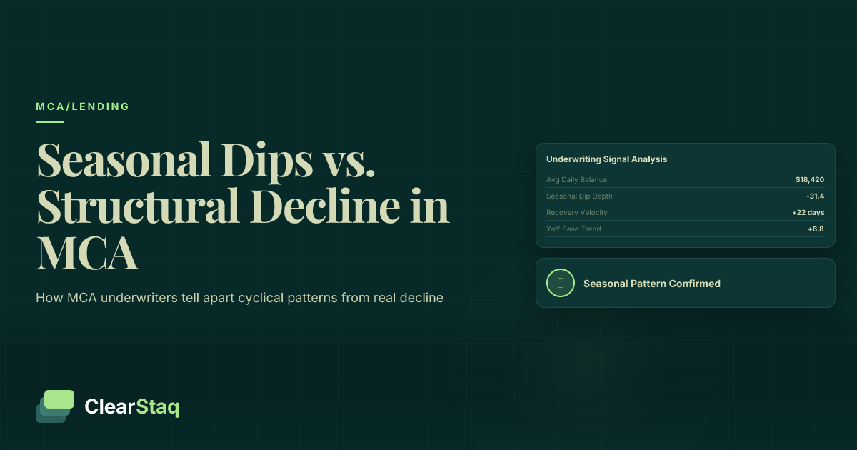
Bank statement seasonality analysis identifies whether a business revenue dip is a predictable cyclical pattern or a sign of structural decline. Underwriters distinguish the two by comparing same-month year-over-year deposits, average daily balance stability, NSF frequency trends, and deposit velocity across a minimum of 24 months of statements — not just the most recent 3 to 6 months.

What Is Bank Statement Seasonality Analysis?

Bank statement seasonality analysis is the process of reading longitudinal cash flow data to determine whether a business's revenue fluctuations follow a predictable, repeating cycle — or whether they reflect something more troubling. For MCA underwriters, this distinction is one of the most consequential judgments in the file.

Most content on this topic is written for borrowers: how to manage slow seasons, how to apply for financing, how to plan ahead. This post is written for the people approving or declining those applications. The analytical problem is different. The stakes are different. And the methodology has to match.

Why MCA Underwriters Face a Different Seasonality Problem Than Traditional Lenders

Traditional bank lenders and SBA programs evaluate businesses using annual financial statements, tax returns, and multi-year P&L summaries. Seasonality smooths out across a 12-month figure. MCA underwriters don't have that luxury.

MCA advances are repaid daily or weekly as a percentage of revenue. That means a seasonal trough directly suppresses repayment velocity — sometimes for months at a stretch. When a landscaping company hits its January low, daily remittances can drop by 60% or more. That's not a loan covenant risk; it's a real-time cash flow event.

Add the time pressure of same-day underwriting decisions, and you have a recipe for two types of errors: approving a declining business that claims seasonality as cover, or declining a perfectly healthy seasonal business that looks distressed on a 3-month snapshot. Both errors are costly. The MCA underwriting checklist addresses how seasonality analysis fits within a broader evaluation framework.

The Difference Between a Seasonal Dip and a Structural Decline

A cyclical dip is predictable, recoverable, and repeating. It occurs at the same point in the calendar each year. Revenue falls, then returns — reliably — to prior-year peak levels or beyond. A structural decline is directional. Revenue falls and doesn't fully recover. Each year's peaks are lower than the last. The trough gets deeper. The pattern is consistent but in the wrong direction.

The challenge is that the same revenue chart can represent either pattern. A January deposit total of $45,000 might be perfectly normal for a pool service company — or it might be a business in freefall. Context and history determine the answer. Five diagnostic signals tell you which is which, and we'll walk through each one.

Why Seasonality Is the Hardest Pattern to Underwrite

Seasonality is invisible unless you have enough data to see it repeat. A single year of statements shows you a curve. Two or three years show you whether that curve is consistent or deteriorating. Most MCA files contain 3 to 6 months of statements. That window captures, at best, one season — and often less than one.

The problem isn't just that 3 months is a small sample. It's that 3 months systematically misleads underwriters toward pessimism or optimism depending on which season the statements happen to cover. A business reviewed in February looks nothing like the same business reviewed in August — even if both reviews are accurate.

No existing analytical framework addresses this problem from the underwriter's perspective. Recognizing what 12 months of bank statements actually show is the minimum starting point — and even 12 months only gives you one full cycle. The reliable standard is 24 to 36 months.

The 3-Month Trap: How Short Data Windows Mislead Underwriters

Consider a landscaping company in the northeastern United States. Its monthly deposit profile might look like this:

Month	Monthly Deposits	Notes
January	$42,000	Deep trough
February	$38,000	Deep trough
March	$71,000	Early recovery
April	$138,000	Ramp up
May	$198,000	Peak season begins
June	$224,000	Peak
July	$218,000	Peak
August	$211,000	Peak
September	$162,000	Late season
October	$94,000	Wind down
November	$58,000	Off-season
December	$47,000	Off-season

If your file contains January, February, and March statements, the trailing 3-month average deposit is approximately $50,333. The business looks weak. A quick capacity calculation produces a small advance offer — or a decline.

If your file contains June, July, and August statements, the trailing 3-month average is approximately $217,667. The same business looks strong, and a much larger advance gets approved. Neither evaluation is wrong given the data. Both evaluations are wrong given the business. Only 24 months of data reveals the truth: this is a $1.6 million annual business with a predictable, healthy seasonal curve.

How External Economic Factors Mask or Mimic Seasonality

Seasonality analysis gets more complicated when macro events enter the picture. A business in genuine structural decline may attribute weak performance to COVID disruption, inflation, or a local economic shift — framing it as an anomalous year rather than a trend. Conversely, a healthy seasonal business may show an unusual year that distorts the pattern due to external factors entirely outside its control.

Underwriters must separate business-specific cycles from macro events. The best method is trailing multi-year data: if a business shows consistent seasonal cycles in 2021 and 2022 but an anomalous dip in 2023, the anomaly warrants a specific explanation — not an automatic assumption of structural decline. The BLS seasonal adjustment methodology provides a useful framework for understanding how economists separate cyclical patterns from trend movements in aggregate economic data — the same logic applies at the individual business level.

The 5 Most Common Seasonal Revenue Patterns in Bank Statements

Every seasonal business has a deposit fingerprint — a characteristic shape that repeats year over year when the business is healthy. Learning to recognize these shapes at the data level is one of the most practical skills an MCA underwriter can develop. Here are the five patterns that appear most frequently in bank statement files.

Pattern 1: Summer Peak. Landscaping, tourism, pool services, outdoor recreation. Strong May through September. Trough October through March. Peak deposits typically 4 to 6 times trough deposits.

Pattern 2: Winter Peak. Retail, gift businesses, holiday-driven services. Strong October through December. Trough January through April. The holiday spike can represent 30 to 40% of annual revenue concentrated in 8 to 10 weeks.

Pattern 3: Tax Season Surge. Tax preparers, accounting practices, H&R Block franchises. Extreme February through April spike. Deposits in peak months may be 8 to 10 times off-season levels. Flat or near-zero deposit activity in summer and fall is entirely normal for this vertical.

Pattern 4: Agricultural Cycle. Farm supply, crop inputs, harvest services. Spring and fall peaks aligned with planting and harvest. Summer and winter troughs. The dual-peak structure can confuse underwriters expecting a single annual cycle.

Pattern 5: Construction and Event-Driven. Revenue tied to project starts rather than calendar months. This pattern is the hardest to model because the peaks don't occur at fixed calendar positions — they shift with project timing, contract awards, and client payment schedules. An underwriter treating construction revenue as seasonal may be misclassifying what is actually lumpy, project-driven cash flow.

Identifying Pattern Type from Deposit Shape Alone

Think of the 12-month deposit bar chart as a waveform. A healthy seasonal business produces a consistent waveform — the same peaks and troughs, roughly the same amplitude, at the same calendar positions each year. When you overlay Year 1, Year 2, and Year 3 on the same chart, the curves should track closely.

Consistent amplitude year over year signals a genuinely seasonal, healthy business. Shrinking amplitude — peaks getting lower while troughs stay flat or get deeper — signals structural deterioration. Shifting peak months — the business's best months occurring earlier or later in the calendar each year — may indicate structural change or external disruption, and warrant a direct conversation with the applicant. For methodology on reading these deposit shapes, see how MCA underwriters read deposit patterns.

Peak Season Leverage: Is the Business Growing Its Peaks Year Over Year?

Peak season leverage is a concept no competitor content covers, but it may be the single most useful diagnostic metric for seasonal business underwriting. The idea is simple: a healthy seasonal business doesn't just repeat its peaks — it grows them, even slightly, over time. Business growth in a seasonal vertical shows up first in the peak months, not the trough months.

To calculate peak season leverage, compare the same peak month across three consecutive years. For a summer-peak landscaping company, compare July deposits in Year 1, Year 2, and Year 3. Flat or growing = healthy trajectory. Declining year over year = early structural warning. The peak months erode before the trough months do in a declining business. That means peak-month decline is the leading indicator — and most underwriters miss it by focusing on trailing averages rather than same-month trend lines.

Cyclical Dip vs. Structural Decline: How to Tell the Difference

This is the core analytical question in seasonal business underwriting, and no existing resource provides an underwriter-specific framework for answering it. The five signals below form a diagnostic system you can apply to any seasonal business file. No single signal is conclusive on its own — the pattern across all five tells the story.

Year-over-Year Same-Month Comparison: The Primary Diagnostic Tool

Pull the deposit total for the same calendar month across three consecutive years and compare them in sequence. This is the most reliable single indicator available in bank statement data.

Month	Year 1 Deposits	Year 2 Deposits	Year 3 Deposits	YoY Trend
January	$44,000	$46,500	$45,200	Flat — cyclical
July (peak)	$198,000	$214,000	$221,000	Growing — healthy

Flat or growing same-month deposits confirm a cyclical pattern. A consecutive decline of more than 10 to 15% in the same month across multiple years is a structural warning signal — particularly if the decline appears in peak months as well as trough months.

This methodology requires 24 or more months of statements. When applicants push back on providing 24 to 36 months of data, the ask is justified: the Federal Reserve Small Business Credit Survey consistently documents that seasonal businesses have materially different financing trajectories than non-seasonal businesses in the same revenue bracket — and they can only be properly evaluated with multi-year data.

NSF Frequency as a Seasonal Health Indicator

NSF activity in bank statements is widely used as a risk signal, but for seasonal businesses the interpretation requires calibration. A small number of NSF events during documented trough months — isolated, predictable, and not worsening year over year — may be acceptable for a business whose peak months show strong cash generation.

The alarming pattern is what underwriters call NSF migration: NSFs that appear earlier in the calendar each year, spreading from deep trough months into months that were previously clean. A business that showed NSFs only in January in Year 1, then January and February in Year 2, then December through February in Year 3 is showing an off-season that is getting longer. That's structural deterioration disguised as seasonal variation. For a detailed methodology on reading NSF patterns, see what NSF frequency reveals about borrower risk.

Average Daily Balance Stability Across Off-Season Months

Standard ADB calculations use the most recent 3 months of statements. For seasonal businesses, this approach is almost meaningless. ADB during a landscaping company's peak season tells you nothing about its financial resilience during January. The metric needs to be segmented.

Calculate ADB separately for peak months and off-season months, then track both across multiple years. The off-season ADB is the diagnostic signal. A healthy seasonal business maintains relatively stable off-season ADB year over year — it has built reserves during peak months, has a line of credit, or has reduced fixed costs enough to survive the slow period without balance erosion.

A declining business shows off-season ADB eroding faster than peak-season ADB. The safety cushion is disappearing. When off-season ADB in Year 3 is 40% lower than Year 1 even though peak deposits are only 10% lower, the business is consuming its reserves to stay alive between seasons. That's a credit risk that a simple trailing ADB calculation won't surface. See the full average daily balance calculation methodology for seasonal business segmentation.

Signal 4: Deposit velocity. Count the number of individual deposits per month — not just the total deposit amount. A healthy seasonal business in its trough may show lower total deposits, but deposit frequency (number of transactions) remains relatively consistent. A declining business shows fewer, smaller deposits because it's losing customers, not just experiencing calendar-driven slow months.

Signal 5: Fixed obligation coverage. Does the business continue to pay rent, payroll, equipment financing, and debt service during the slow season? If yes, the off-season is manageable. If the bank statements show these obligations being deferred, missed, or paid late — particularly in previously clean months — the business is struggling to service its fixed costs even before the advance is added to the picture.

Industry-by-Industry Seasonality Benchmarks

Understanding what a normal seasonal pattern looks like for a specific vertical is what separates a competent underwriter from an exceptional one. The benchmarks below define the expected pattern — so abnormal variations are immediately visible.

Landscaping and Lawn Care: Q1 Trough Is Expected, Not Alarming

For most US geographies, landscaping revenue drops 60 to 75% from peak during January and February. A January deposit total that is 25 to 30% of the prior July or August peak is entirely normal. The recovery typically begins in April and reaches full run rate by May.

The red flag is January deposits falling below 15% of the summer peak — particularly if that ratio is worsening year over year. This pattern suggests the business isn't just experiencing winter; it's losing accounts and failing to rebuild its client base each spring. Secondary checks include equipment financing payments (are they continuing through the winter, indicating the business is maintaining assets?) and payroll activity (is there a consistent core crew being paid year-round, or has the business laid off everyone and gone dark?).

Retail and Gift Businesses: The Holiday Spike and Q1 Hangover

November and December often represent 30 to 40% of annual revenue for a traditional retail business. The Q1 trough that follows is structurally expected — it's the hangover after the holiday surge, not a sign of weakness. The diagnostic focus should be on whether the Q1 trough is stable or worsening year over year.

The critical red flag is peak month erosion: if November and December deposits are declining year over year while Q1 remains equally depressed, the business is losing holiday market share. It's not recovering to prior-year peaks in its best months. That's the leading indicator of structural decline in retail. Note that e-commerce retailers typically show a much smoother revenue curve than brick-and-mortar stores. Dramatic seasonality in a business described as primarily e-commerce warrants investigation — it may indicate something other than calendar-driven patterns.

Restaurants: Daily Deposits That Mask Seasonal Complexity

Restaurants present a layered seasonality problem. They have micro-seasonality — weekday versus weekend deposit patterns — layered on top of macro-seasonality tied to summer patio traffic, holiday dining, and local events. Monthly deposit totals can be highly variable based on how many weekends fall in a given month.

Before assessing monthly revenue trends, normalize restaurant deposits by day-of-week frequency. A month with five Saturdays is not comparable to a month with four. The most reliable signal is the average daily deposit size over rolling 4-week windows — this strips out calendar effects and reveals true volume trends. For detailed methodology on restaurant deposit pattern analysis, see our restaurant cash flow analysis. Red flag: declining average daily deposit size over 6 or more consecutive months signals customer volume loss that is not seasonal in nature.

Construction: Project-Driven Cash Flow That Mimics Seasonality

Construction revenue is project-driven, not calendar-driven — but it can appear seasonal because project starts are loosely correlated with weather and fiscal year cycles. Underwriters who treat construction cash flow as seasonal are making a category error.

For construction businesses, focus on consistent annual revenue totals rather than monthly distribution. The monthly pattern will always be lumpy; the question is whether total annual deposits are stable, growing, or declining across consecutive years. The most useful forward-looking indicator is payment gap analysis: how long between the completion of one project (large incoming lump-sum deposit) and the start of the next? If those gaps are getting longer year over year, the pipeline is thinning — a structural signal regardless of how the monthly deposit chart looks.

Key Bank Statement Metrics for Seasonal Business Analysis

The framework below consolidates the signals discussed throughout this post into a reference set that can be applied systematically to any seasonal business file.

Metric	What It Measures	Healthy Signal	Warning Signal
Same-month YoY deposit delta	Revenue trend at the same seasonal position	Flat or positive	Declining >10% consecutively
Peak-month deposit trend (3 years)	Peak season leverage	Growing or flat	Declining in peak months first
Off-season ADB stability	Reserve cushion and fixed cost coverage	Declining less than 10% YoY	Eroding faster than peak ADB
NSF migration calendar	Whether problem months are expanding	NSFs limited to deep trough months	NSFs spreading into peak months
Deposit frequency (count)	Customer volume trend	Consistent count, variable amounts	Fewer deposits even if amounts hold
Fixed obligation coverage	Can the business service costs off-season?	Rent, payroll, debt service paid on time	Deferrals, missed payments in trough

How to Weight Peak vs. Off-Season Revenue in Capacity Calculations

The most common mistake in seasonal business underwriting is using a trailing 3-month average to calculate advance capacity when that window falls during the trough. The result is an artificially suppressed offer that doesn't reflect the business's true annual capacity — and may price a creditworthy applicant out of the market.

A better approach is a weighted annual average. For a landscaping business with 4 strong peak months and 8 slower months, weight the peak period at 70% and the off-season at 30% of the annual capacity calculation. This produces an advance amount grounded in total annual throughput rather than a seasonally distorted snapshot. The advance can then be stress-tested against off-season cash flow: can the business cover daily remittances at the proposed percentage even during its slowest months? That's the floor. Understanding how bank statement velocity predicts repayment success is essential for calibrating this calculation correctly.

Red Flags That Indicate Seasonality Is Being Used as an Excuse

Experienced underwriters develop pattern recognition for applicants who invoke seasonality to explain what is actually structural decline. The signals below — particularly when two or more appear together — should trigger deeper scrutiny:

• Peak months are declining year over year, not just the trough (businesses in genuine seasonal decline show peak erosion before trough deepening)
• NSF fees appear during what should be the business's strongest revenue months
• Average daily balance in peak months is declining even as the owner reports strong seasonal performance
• Deposit count is declining even if deposit amounts are holding steady — fewer customers, each spending more, represents revenue concentration risk
• No evidence of reserves accumulated during peak season: the balance resets to near-zero each fall, with no buffer carried into the off-season
• The business has a history of MCA advances taken at the start of each trough — potentially a sign of a cash-flow-dependent operation rather than a genuinely seasonal one

How Automated Analysis Changes the Seasonality Equation

The methodology described in this post is analytically sound — and operationally burdensome when done manually. A 36-month seasonality analysis for a single file means pulling 36 separate bank statement PDFs, building a structured spreadsheet, calculating same-month YoY comparisons, segmenting ADB by season, tracking NSF migration, and comparing the result against industry benchmarks. That's 2 to 4 hours of analyst time per file. At scale, it's impractical.

Automated bank statement analysis changes what's operationally feasible. When processing time drops from hours to seconds, underwriters can request 24 to 36 months of statements as a standard rather than an exception. That data standard — not the analysis methodology itself — is what makes reliable seasonality classification possible. No competitor content addresses automation in the context of seasonality analysis. This is a gap that directly affects underwriting quality across the MCA industry.

What ClearStaq's Seasonality Analysis Actually Does

ClearStaq's MCA underwriting platform processes multi-statement batches in seconds, not hours. Upload 24 to 36 months of bank statements and receive a structured longitudinal analysis that includes:

• Automated year-over-year same-month deposit comparison with directional trend flagging (growing, flat, or declining)
• Industry vertical tagging that surfaces sector-specific seasonal norms for comparison against the applicant's actual pattern
• ADB trend analysis segmented by configurable time windows — peak months versus off-season months — tracked across all uploaded periods
• Deposit velocity and frequency metrics tracked across the full multi-year data set
• NSF migration mapping that shows which calendar months have shown NSF activity across consecutive years
• MCA stacking detection to identify whether a seasonal business is entering peak season already over-leveraged from advances taken during the trough

The output is a seasonality classification — confirmed seasonal, inconclusive, or structural decline signal — with the supporting metrics that justify the classification. Underwriters get a decision-ready analysis, not a stack of PDFs.

From Manual Review to Automated Seasonal Pattern Recognition

The workflow comparison is stark. Manual review of a 36-month file: pull each PDF individually, extract monthly deposit totals, build a comparison spreadsheet, calculate YoY deltas, segment ADB by season, plot NSF timing, look up industry benchmarks, write the credit memo finding. Two to four hours minimum, with meaningful risk of calculation error.

Automated review: upload the batch. Receive structured output — deposit curves, trend flags, ADB segmentation, NSF migration map, industry comparison — in seconds. The underwriter's job shifts from data extraction to interpretation and judgment. That's where human expertise belongs.

AI pattern recognition adds a layer that manual analysis can't replicate at any speed: matching the applicant's deposit curve against a library of known seasonal signatures to determine whether the pattern is consistent with the claimed industry cycle, or whether it shows deterioration characteristics that don't fit the seasonal explanation.

Adjusting MCA Offer Structures for Seasonal Businesses

Once you've confirmed that a business is genuinely seasonal rather than structurally declining, the question shifts from whether to fund to how to structure the advance. Standard MCA offer structures — fixed daily remittance as a percentage of deposits — create predictable stress for seasonal businesses during trough months. Structuring the advance correctly is what separates a performing deal from a default.

Remittance Percentage Strategies for Seasonal Cash Flow

A fixed remittance percentage works well for businesses with consistent monthly cash flow. For a verified seasonal business, the same structure can impose crushing daily obligations during months when deposits are 25% of peak levels. The math often doesn't work — and the business either defaults or returns for a new advance to cover the old one.

For seasonal businesses, consider these structural approaches:

• Variable remittance structure: Higher percentage during documented peak months (when the business can afford it), lower percentage during documented trough months. This requires a clear contractual definition of peak and off-season months based on the historical data.
• Minimum dollar floor: Some MCA providers set a minimum daily dollar amount rather than a percentage. This protects advance performance but can create hardship during deep troughs if the floor is set too high relative to off-season cash flow.
• Peak-season funding timing: The safest structural choice is timing: fund the advance at the start of the business's peak season, not mid-trough. Early repayments are strong, exposure decreases rapidly, and the advance may be substantially paid down before the next trough begins.

Advance amount sizing follows the same principle: use peak-season capacity as the ceiling, stress-test repayment against off-season cash flow as the floor. An advance that the business can service even in its worst month is a performing deal. An advance that requires peak-month revenue to stay current is a seasonal time bomb.

How to Document Seasonal Classification in the Underwriting File

Formal documentation of the seasonality finding protects the underwriter, supports the advance pricing decision, and creates an audit trail if the advance performs differently than projected. The credit memo should include:

• Seasonal pattern type (summer peak, winter peak, tax season surge, etc.)
• Number of months analyzed and date range of statements reviewed
• Year-over-year trend direction for same-month deposits (growing, flat, or declining — with specific figures)
• Peak season leverage calculation: are peaks growing, flat, or declining across the three most recent peak periods?
• Industry benchmark comparison: how does the applicant's seasonal pattern compare to the typical pattern for its vertical?
• Any external factors that may have distorted a specific year's data (COVID, local disasters, supply chain disruption)
• Seasonality classification: confirmed seasonal, inconclusive, or structural decline signal

This documentation makes the underwriting rationale transparent and reproducible. If the advance performs differently than projected, the file shows exactly what information was available, how it was analyzed, and what conclusion was reached — and why.

FAQ: Seasonality Analysis in MCA Underwriting

How do you identify seasonal patterns in bank statements?

Identify seasonal patterns by comparing same-month deposits across at least 24 months of bank statements. A genuine seasonal business shows a consistent, repeating revenue curve — with peak and trough months occurring at the same points in the calendar each year. Automated analysis tools can plot this pattern instantly across multi-year data, flagging whether the curve is stable, growing, or deteriorating.

What is the difference between a cyclical dip and a declining business?

A cyclical dip is a predictable, repeating revenue reduction that occurs at the same time each year and recovers to prior-year peak levels. A structural decline shows year-over-year deterioration in same-month deposits, shrinking peak-season revenue, and increasing NSF frequency — often appearing in months that were previously clean. The key diagnostic is whether peak months are growing, flat, or declining across consecutive years. Peak erosion is the leading indicator of structural decline.

How many months of bank statements are needed to detect seasonality?

A minimum of 24 months is required to detect genuine seasonality, and 36 months is the recommended standard for MCA underwriting. Three to six months of statements — the most common MCA request — are insufficient for reliable seasonality analysis and can cause underwriters to misclassify a healthy seasonal business as high-risk, or to approve a declining business that points to seasonality as cover for structural weakness.

How do MCA lenders handle seasonal businesses?

MCA lenders evaluate seasonal businesses using year-over-year deposit comparisons, average daily balance stability across peak and off-season months, and peak season leverage analysis. Offer structures for verified seasonal businesses may include variable remittance percentages tied to revenue performance, or advance timing aligned with the start of peak season to maximize early repayment strength and reduce exposure before the trough begins.

What industries have the most seasonal cash flow variation?

Industries with the highest seasonal cash flow variation in MCA bank statement files include landscaping and lawn care, retail and gift businesses, tax preparation services, agriculture-related businesses, and tourism and hospitality. Construction businesses show significant monthly cash flow variation as well, though theirs is often project-driven rather than calendar-driven — making it harder to model as a true seasonal pattern and requiring a different analytical approach.

What cash flow metrics reveal true business health in seasonal industries?

The most reliable metrics are same-month year-over-year deposit delta, peak-month deposit trend across three consecutive years, off-season average daily balance stability, NSF frequency migration across the calendar, and deposit count per month. A healthy seasonal business maintains stable or growing peaks, consistent off-season ADB, and NSF activity limited to trough months rather than spreading into peak or shoulder months year over year.