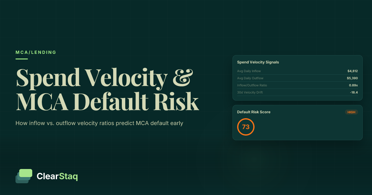
Transaction Velocity Analysis: Using Spend Rate Data to Predict MCA Default Risk

Transaction velocity — the rate at which money moves into and out of a merchant's account over a defined period — is a leading indicator of MCA default risk. By calculating inflow velocity, outflow velocity, and the ratio between them from raw bank statement data, underwriters can identify deteriorating repayment capacity 30 to 60 days before a default occurs, well ahead of traditional credit signals.

What Is Transaction Velocity and Why MCA Lenders Should Care

Transaction velocity is not a new concept in finance, but it's an underused one in MCA underwriting. It describes the rate and rhythm of money moving through a business bank account over time — not just how much arrives, but how fast it arrives, how fast it leaves, and what remains in between.

Most MCA underwriters still rely on monthly revenue totals, average daily balance, and FICO scores to assess default risk. These are useful signals, but they're lagging indicators. By the time a declining FICO score reflects a merchant's deteriorating financial position, the default is often weeks away. According to the Federal Reserve Small Business Credit Survey, a significant share of small businesses that seek alternative financing are already experiencing cash flow stress — meaning the problem existed long before traditional credit metrics flagged it.

Transaction velocity changes that. It gives underwriters a forward-looking lens built from the same bank statement data they're already reviewing — just analyzed with more precision.

Velocity vs. Volume: Why the Distinction Matters

Volume and velocity are easy to confuse, but the distinction is critical for repayment risk assessment.

Consider two restaurants applying for an MCA. Restaurant A posts $80,000 in monthly revenue. Restaurant B posts $50,000. On volume alone, Restaurant A looks stronger. But if Restaurant A's outflow velocity consumes 95% of that revenue, it has a daily net cash buffer of roughly $133. Restaurant B, spending only 60% of its revenue, generates a daily net buffer of $667.

The MCA holdback is a fixed daily percentage of revenue. Velocity determines whether that percentage is sustainable. Volume tells you what came in. Velocity tells you how fast it left — and whether anything meaningful remains to cover the advance.

Why Traditional Credit Metrics Miss Velocity Signals

FICO scores reflect historical payment behavior. They update slowly and don't capture what's happening inside a business account right now. A merchant can have a 680 FICO score and a catastrophically fast cash burn rate — and no credit bureau signal will surface that risk in time.

Monthly revenue figures are averages that hide intra-month dynamics. A merchant showing $60,000 average monthly revenue might have earned $85,000 in Month 1, $60,000 in Month 2, and $35,000 in Month 3. The average looks acceptable. The trajectory is alarming.

Research consistently shows that bank statement velocity predicts repayment success in ways that credit scores cannot. The signal is embedded in the transaction data — it just needs to be extracted correctly.

The Three Velocity Signals That Predict Default Risk

Effective transaction velocity MCA risk analysis is built on three discrete signals, each derived from transaction-level bank statement data. No single signal is sufficient on its own. The relationship between all three is what makes the framework predictive.

Inflow Velocity: Measuring Revenue Momentum

Inflow velocity is defined as total credit transaction value divided by the number of business days in the period. It expresses how much revenue, on average, enters the account each business day.

The key threshold: when inflow velocity drops more than 20% month-over-month for two consecutive months, flag the application for elevated review. A single-month dip may reflect a seasonal trough or a one-time disruption. Two consecutive months of decline signal a structural change in revenue momentum.

Inflow velocity also behaves very differently across merchant types. Understanding recurring vs. lumpy revenue deposit patterns matters here — a retail merchant with daily card transactions shows smooth, consistent inflow velocity, while a contractor receiving project payments shows irregular spikes that can artificially inflate or suppress the average.

One technical note: duplicate ACH credits — double-counted deposits that sometimes appear in raw statement exports — can inflate inflow velocity. Automated deduplication is not optional; it's a data integrity requirement for accurate velocity analysis.

Outflow Velocity: Measuring Cash Burn Rate

Outflow velocity is total debit transaction value divided by the number of business days in the period. It expresses the daily rate at which money leaves the account.

The primary pre-default pattern is straightforward: rising outflow velocity against flat or declining inflow velocity. When a merchant is spending faster than they're earning — and that gap is widening — repayment capacity is deteriorating in real time.

Blunt outflow totals are less useful than categorized outflow. Knowing that a merchant is spending $800 per day tells you little. Knowing that $300 of that is payroll, $150 is rent, $200 is supplier payments, and $150 is existing MCA repayments tells you everything about their cost structure and flexibility.

High outflow velocity frequently co-occurs with deteriorating account health. NSF fees and negative balance days tend to spike in parallel with outflow velocity increases — both are symptoms of the same underlying cash flow compression.

Net Velocity: The Repayment Capacity Ratio

Net velocity is inflow velocity minus outflow velocity, expressed as a daily net cash generation rate. This is the number that matters most for MCA repayment sustainability.

The logic is simple: net velocity must exceed the MCA daily holdback amount for repayment to be sustainable. If it doesn't, default is a mathematical inevitability — the only question is timing.

Consider a concrete example. A merchant has a net velocity of $420 per day and a proposed holdback of $380 per day. The buffer is $40 — roughly a 10.5% margin. A 10% revenue dip eliminates that buffer entirely. That merchant is one slow week away from a missed payment.

Net velocity trending toward zero is the clearest pre-default signal available from bank statement data. It doesn't require modeling or inference — it's visible in the arithmetic.

The chart above illustrates how inflow, outflow, and net velocity track across a 90-day window. Notice how net velocity compression becomes visible weeks before it reaches zero — this is the pre-default window that trajectory analysis is designed to catch.

Inflow vs. Outflow Velocity: Reading the Ratio That Matters Most

The inflow-to-outflow velocity ratio (I/O ratio) synthesizes both signals into a single number that expresses repayment capacity as a multiplier. It's the most actionable metric in velocity-based MCA underwriting.

I/O Ratio Range	Risk Classification	Recommended Action
1.30 and above	Healthy — low default risk	Standard underwriting process
1.10 to 1.29	Watch-list — elevated risk	Human review, trajectory analysis required
Below 1.10	High default risk	Decline or significantly reduced offer

One critical nuance: a declining I/O ratio trend is a warning signal even when the absolute ratio is still above 1.0. A merchant at 1.15 today but 1.45 three months ago is burning through their buffer. The ratio may still look technically acceptable. The direction is not.

Before computing the I/O ratio, strip existing MCA repayment debits from the outflow total. Including them inflates apparent outflow velocity and underestimates available cash flow for a new position. The average daily balance calculation serves as a useful cross-check: average daily balance and net velocity should move in the same direction. If they diverge, investigate why.

How to Interpret I/O Ratio Compression

I/O ratio compression refers to the ratio narrowing toward 1.0 over successive months, even while the merchant remains nominally cash-flow positive. It's the financial equivalent of watching a fuel gauge slowly approach empty.

Compression sustained over 60 days is a high-confidence pre-default signal. The merchant is burning through their buffer faster than they're rebuilding it. Each month, less remains to absorb the inevitable revenue fluctuation.

One important exception: seasonal businesses. A restaurant's I/O ratio will compress naturally in January and February as winter traffic slows. Penalizing that compression without seasonal context produces false positives. Always consult seasonality analysis in bank statements before flagging cyclical compression as structural default risk.

Worked Example: Reading the I/O Ratio from Raw Data

Here's a three-month velocity analysis for a single merchant application:

Month	Total Credits	Total Debits	I/O Ratio	Signal
Month 1 (oldest)	$71,000	$50,000	1.42	Healthy
Month 2	$65,000	$53,700	1.21	Watch-list
Month 3 (most recent)	$62,000	$57,400	1.08	High risk

The absolute ratio in Month 3 is 1.08 — above 1.0, meaning the merchant is still technically cash-flow positive. But the trajectory is unambiguous: the I/O ratio has dropped 0.34 points in 60 days. Without intervention, Month 4 likely falls below 1.0.

Now apply the MCA-repayment strip. If $8,000 of the Month 3 debit total represents an existing advance repayment, the adjusted outflow is $49,400 and the adjusted I/O ratio climbs to 1.25. That changes the picture significantly for a second-position analysis — the operational business is less distressed than the raw numbers suggest, but the existing advance is consuming the margin.

How to Calculate Spend Rate from Raw Bank Statement Data

Spend rate analysis translates raw transaction data into a usable underwriting metric. Here's the step-by-step methodology your team can apply to any bank statement:

1. Separate credit and debit transactions by date. Do not use statement-level totals. Pull the transaction-level data. Statement totals can aggregate across sub-periods in ways that obscure intra-month velocity patterns.
2. Remove non-operational transactions. Exclude transfers between the merchant's own accounts, loan proceeds, tax refunds, and one-time insurance settlements. These inflate credits without reflecting genuine revenue velocity.
3. Calculate daily averages for credits and debits across the statement period by dividing totals by business days, not calendar days.
4. Compute the spend rate as (total debits ÷ total credits) × 100. This expresses, as a percentage, how much of incoming revenue is consumed by outgoing expenses. A spend rate of 75% means 25 cents of every dollar earned remains — the buffer available for debt service.
5. Repeat across 3 to 6 months and chart the trajectory. A single-period spend rate is a snapshot. The trend across periods is the predictive signal.

The practical challenge: manual calculation across the hundreds of bank formats that appear in an MCA application pipeline is slow and error-prone. Format inconsistencies — how Chase exports transaction descriptions vs. how a regional credit union does — create normalization problems that compound at scale.

Transaction Categorization: Why Blunt Totals Mislead

Spend rate becomes significantly more powerful when outflow is categorized rather than aggregated. Breaking debits into labeled buckets — payroll, rent, supplier payments, MCA repayments, taxes, utilities — reveals the cost structure underneath the total.

The key risk distinction is fixed vs. variable costs. A merchant with 80% of outflow velocity tied to fixed costs (rent, payroll, existing debt service) has almost no ability to reduce spending if revenue drops. Their spend velocity is structurally rigid. A merchant with 60% variable cost outflow can cut spending quickly when revenue falls — their repayment risk profile is materially different.

MCA repayment debits require special handling. They must be identified, labeled separately, and excluded from the operational spend rate calculation. Treating them as organic business expenses overstates the cost burden of running the business and understates the burden of existing debt service — two different problems that require different responses.

How Many Months of Data Are Needed for Reliable Velocity Analysis

The answer depends on what you're trying to measure:

• 3 months (minimum viable): Establishes a baseline. Reveals the current velocity level but provides only one period of comparison — not enough to confirm a trend direction with confidence.
• 6 months (recommended standard): Reveals one clear trend direction. Sufficient to distinguish a structural decline from a temporary dip. This is the recommended standard for most MCA applications.
• 12 months (optimal): Enables full seasonality normalization. Identifies whether a velocity decline is cyclical (expected to recover) or structural (unlikely to recover). The SBA's small business economic profile documents significant cash flow volatility among small businesses — 12 months of data is the only way to reliably distinguish volatility from deterioration.

Single-month velocity readings have limited predictive value regardless of what they show. A snapshot tells you where a merchant stands today. Only a trajectory tells you where they're heading.

Velocity Trending: Snapshots vs. Trajectories in Risk Scoring

The most important conceptual shift in velocity-based underwriting is this: the trajectory of velocity matters more than any single reading.

A merchant with an I/O ratio of 1.15 today is a fundamentally different risk depending on direction. If that ratio was 1.05 three months ago, the merchant is improving — their repayment buffer is growing. If that ratio was 1.45 three months ago, the merchant is deteriorating — their buffer is shrinking at a rate that will breach sustainable levels within weeks.

Same number. Opposite risk profiles. A snapshot-only underwriter would treat them identically. A trajectory-aware underwriter would make very different decisions.

The 60-Day Pre-Default Velocity Pattern

Analysis of MCA defaults reveals a consistent velocity pattern in the 60 days preceding a missed payment:

• Inflow velocity begins declining — typically 15 to 25% below the prior period average
• Outflow velocity holds steady or increases — fixed costs continue while revenue compresses
• Net velocity collapses toward zero or turns negative
• NSF frequency increases, often doubling in the final 30 days before default
• Average daily balance shows late-month compression — the account is being run down to near-zero by month's end

Critically, this pattern is only detectable through trajectory analysis. An underwriter reviewing only the most recent month's statement would see declining revenue — concerning, but not necessarily alarming. The same underwriter reviewing six months of velocity data would see a pattern that has been building for two months and is unlikely to reverse without a significant operational change.

Weighting Recent Months in Velocity Scoring

Not all months in a multi-period analysis carry equal predictive weight. Current trajectory is more predictive than historical baseline. A practical weighted scoring approach:

• Month 3 (most recent): 50% weight
• Month 2: 30% weight
• Month 1 (oldest): 20% weight

This weighting ensures that a merchant showing strong historical velocity but sharp recent deterioration receives a risk score that reflects current trajectory, not past performance. Automated systems can apply this weighting consistently across every application. Manual review rarely does — underwriters naturally anchor to the most salient number they see, which may not be the most predictive one.

Velocity trajectory scoring works best as one input into a complete underwriting decision. Pair it with your MCA underwriting checklist to ensure velocity signals are evaluated alongside deposit pattern analysis, NSF frequency, industry context, and time in business.

Industry-Specific Velocity Benchmarks for MCA Underwriters

Velocity thresholds are not universal. The same I/O ratio that signals high risk in a professional services firm is entirely healthy for a restaurant. Industry context changes the risk interpretation significantly — and applying universal thresholds produces systematic errors in both directions.

Restaurants and Food Service

Food service businesses operate with high daily transaction frequency and high outflow velocity relative to revenue. Food costs, labor, and lease obligations consume a large share of every dollar earned. A healthy I/O ratio floor for restaurants is lower than most other verticals — approximately 1.1 to 1.2 is acceptable, where 1.1 to 1.3 would be a watch-list threshold for other industries.

Inflow velocity for restaurants is typically stable and granular — many small card transactions throughout the day. But tip pooling, split-tender payments, and third-party delivery platform deposits (which arrive on payout schedules, not daily) create noise in inflow velocity calculations. Understanding restaurant cash flow deposit patterns is essential before interpreting velocity readings for this vertical.

Seasonal compression in January and February is normal and expected. Don't penalize a restaurant for predictable post-holiday slowdown without applying seasonal adjustment first.

E-Commerce and Retail

E-commerce merchants receive revenue through platform payout schedules — Shopify, Amazon, Stripe, and similar platforms typically disburse weekly or bi-weekly, not daily. This creates lumpy inflow velocity that doesn't reflect actual sales velocity. Evaluate I/O ratios for e-commerce on a weekly basis rather than daily to align with the actual payout cadence.

Holiday inventory buildup creates legitimate outflow velocity spikes in October and November. An e-commerce merchant increasing supplier payments sharply in Q4 isn't necessarily deteriorating — they may be building inventory ahead of a high-revenue period. Without context, this pattern triggers a false positive.

Chargebacks and returns create inflow velocity reversals that must be netted out. Platform-level refunds can appear as debit transactions that inflate outflow velocity or as reduced credit transactions that suppress inflow velocity, depending on how the platform processes them.

Service Businesses and Professional Services

Professional services firms — consultancies, legal practices, marketing agencies — operate with lower transaction frequency and more project-driven, lumpy inflow velocity. Outflow velocity is also lower than retail because there's minimal cost of goods sold. The healthy I/O ratio floor for this vertical is higher: 1.4 or above should be the minimum threshold.

Payroll is the dominant risk driver in outflow velocity for service businesses. When payroll represents 60% or more of outflow velocity, any revenue disruption immediately threatens both debt service and personnel costs simultaneously.

Month-end invoice clustering creates artificial inflow velocity spikes. A firm that bills on net-30 terms may receive the majority of its monthly revenue in the first few business days of each month, skewing daily inflow velocity calculations. Average the inflow across the full billing cycle before computing velocity ratios.

How Transaction Velocity Reveals MCA Stacking Before It's Disclosed

MCA stacking — taking multiple advances from different lenders simultaneously without disclosing the other positions — is consistently cited as one of the top drivers of MCA default. DeBanked's MCA industry data identifies stacking as a primary factor in a significant share of portfolio losses. The problem is that merchants rarely disclose all positions voluntarily.

Transaction velocity analysis reveals stacking without requiring disclosure. It appears in the outflow data as a pattern of regular, fixed-amount, high-frequency debits — typically daily, typically between $200 and $2,000 depending on advance size. This is the velocity signature of an existing MCA repayment obligation.

The Velocity Signature of Hidden MCA Positions

A merchant with one disclosed MCA position shows one series of consistent daily debits from a known lender. A merchant with two or three positions — one disclosed, others hidden — shows multiple overlapping series of fixed daily debits. The total debt service outflow velocity tells the story even when the merchant doesn't.

The diagnostic threshold: if identifiable fixed daily debits represent more than 30% of inflow velocity, the merchant is likely over-leveraged regardless of what they've disclosed. At that level, the debt service burden alone — before a single operational expense is paid — consumes nearly a third of revenue.

Automated MCA position detection can label these debits before velocity calculations are run, producing a clean separation between debt service outflow velocity and operational outflow velocity. This is far more reliable than asking merchants to self-report their existing obligations.

When velocity patterns suggest undisclosed positions, escalate immediately to a full analysis. Learn how to detect MCA stacking from bank statements using the complete detection methodology.

Adjusting Velocity Analysis for Existing Positions

Once existing MCA repayment debits are identified and labeled, compute two separate velocity figures:

1. Operational outflow velocity: total debits minus identified MCA repayments, divided by business days
2. Debt service outflow velocity: identified MCA repayments only, divided by business days

Then calculate available net velocity: inflow velocity minus total outflow velocity (operational plus debt service). This is the true repayment capacity for any new advance being considered.

If available net velocity after existing positions is less than the proposed new holdback amount, decline — regardless of gross revenue, regardless of stated monthly deposits. The arithmetic doesn't leave room for another obligation. This calculation is the most direct link between velocity analysis and factor rate and holdback optimization.

Automating Velocity Analysis: From Manual Spreadsheets to API-Driven Scoring

The manual approach to velocity analysis is familiar to most MCA underwriting teams: export transactions from a PDF bank statement, paste into Excel, build formulas to separate credits and debits, compute averages, flag anomalies. Repeat for each of six months. Repeat for each application.

This process takes 45 to 90 minutes per application at a minimum. It produces inconsistent results across underwriters. And it breaks down entirely when statements arrive in unfamiliar formats — which happens constantly across a portfolio that spans hundreds of banks and credit unions.

The scalability ceiling is severe. Manual velocity analysis limits throughput to a handful of applications per day per underwriter. For any MCA funder trying to make same-day decisions at volume, that's not a process — it's a bottleneck.

What Automated Parsing Enables That Manual Review Cannot

The ClearStaq MCA underwriting platform addresses the scale problem with API-driven bank statement parsing. Submit a statement, receive structured velocity data in under 60 seconds — across 900+ bank formats, with no manual normalization required.

Specifically, automation enables:

• Duplicate transaction detection — prevents inflated inflow velocity from double-counted ACH credits that appear in some bank export formats
• Automated transaction categorization — breaks outflow velocity into labeled buckets (payroll, MCA repayments, rent, suppliers) without manual line-by-line review
• Multi-period trajectory analysis — computes velocity metrics across 6 to 12 months of statements simultaneously, not sequentially
• Integrated fraud detection — velocity anomalies and 27 fraud signals are computed in a single API call, not separate workflows

Understanding how fintech lenders use bank statements to build risk scores illustrates why velocity analysis fits naturally into automated underwriting pipelines rather than manual review queues.

Building Velocity Analysis Into Your Underwriting Workflow

A practical integration pattern for MCA funders:

1. Applicant uploads bank statements via document portal at application time
2. API parses statements and returns structured JSON with categorized transactions, velocity metrics, and MCA position flags
3. Underwriting system ingests velocity scores automatically and routes the application accordingly
4. High-confidence approvals proceed through automated decisioning; flagged applications route to human review with velocity data pre-loaded

Webhook delivery means velocity data is available before the underwriter opens the file — not after manual extraction. This eliminates the 24 to 48 hour delay between application receipt and velocity analysis that manual review creates. For a same-day decision workflow, that gap is the difference between winning and losing the deal.

Building a Velocity-Based Default Risk Score

The velocity signals described throughout this article become most powerful when synthesized into a single composite score that underwriters can act on directly. Here's a practical scoring framework that combines the key velocity inputs into a 0-to-100 risk score.

A Practical Velocity Scoring Framework

Score Component	Maximum Points	What It Measures
I/O Ratio (3-month weighted average)	40 points	Ratio level and trajectory direction
Net Velocity vs. Proposed Holdback	30 points	Buffer margin above daily holdback amount
Velocity Trajectory	20 points	Whether trend is improving, flat, or declining
Debt Service Ratio	10 points	Percentage of outflow velocity consumed by existing MCA repayments

Score interpretation:

• 75 to 100: Low risk — standard underwriting process applies
• 50 to 74: Moderate risk — human review required, additional documentation may be requested
• Below 50: High risk — decline, or significantly reduced offer with intensified monitoring

Mapping Velocity Scores to Factor Rates and Holdback Percentages

The velocity score's operational value comes from connecting it directly to pricing decisions — something no current competitor framework addresses explicitly.

• High velocity scores (75+): Factor rate at the lower end of your range, standard holdback percentage (typically 10-12%). The merchant's buffer is sufficient to absorb normal revenue fluctuation.
• Moderate velocity scores (50-74): Factor rate adjusted upward by 0.05 to 0.15 to compensate for elevated risk. Holdback percentage lowered slightly to reduce daily cash burden — a lower holdback reduces default probability even as the factor rate adjusts for risk.
• Low velocity scores (below 50): Decline, or offer a significantly reduced advance amount at a higher factor rate with weekly monitoring of velocity metrics post-funding.

This connection between velocity score and pricing is the operational output that makes the entire framework actionable. Velocity analysis without a pricing decision rule is academic. With pricing decision rules, it becomes a competitive underwriting advantage.

Pair velocity scoring with debt service coverage ratio analysis for a complete picture. DSCR and velocity scoring address overlapping but distinct dimensions of repayment risk — together, they provide a more complete underwriting framework than either metric alone.

Frequently Asked Questions

What is transaction velocity in lending risk assessment?

Transaction velocity measures the rate at which money flows into and out of a business bank account over a defined period. In MCA lending, underwriters use inflow velocity, outflow velocity, and the ratio between them to assess whether a merchant generates enough daily net cash to sustain advance repayments — making it a leading indicator of default risk that traditional credit metrics can't replicate.

What cash flow patterns indicate MCA default risk?

The clearest pre-default velocity pattern is inflow velocity declining while outflow velocity holds steady or rises, causing net velocity to compress toward zero. This pattern typically emerges 30 to 60 days before a default event and is most visible through trajectory analysis across three to six months of bank statement data. A single-period snapshot will miss it entirely.

What is the difference between revenue velocity and spend velocity?

Revenue velocity (inflow velocity) measures the daily rate of credit transactions entering the account — how fast money comes in. Spend velocity (outflow velocity) measures the daily rate of debit transactions leaving the account. The ratio between them determines repayment capacity: a merchant with high revenue velocity but equally high spend velocity has little buffer to sustain MCA holdbacks, regardless of gross revenue.

How many months of bank statements do MCA lenders typically review for velocity analysis?

A minimum of three months establishes a baseline, but six months is the recommended standard for reliable velocity analysis because it reveals one directional trend with statistical confidence. Twelve months is optimal when seasonality normalization is needed. Single-month velocity readings have limited predictive value because they capture only a snapshot, not a trajectory.

Can transaction velocity replace credit score in MCA underwriting?

Transaction velocity analysis doesn't replace credit scoring — it serves as a more timely complement to it. Credit scores reflect historical behavior and update slowly. Velocity analysis is derived from current bank statement data and can detect deteriorating repayment capacity weeks before it shows up in credit bureau data. Most sophisticated MCA underwriters use velocity metrics as the primary signal and credit score as a secondary qualifier.