Revenue Seasonality Mapping: How CPAs Benchmark Client Cash Flow Month Over Month

Revenue seasonality mapping is the process of analyzing 12 to 24 months of bank statement data to identify a client's recurring cash flow peaks, troughs, and transition months. CPAs use it to build month-over-month benchmarks, distinguish true seasonal patterns from business decline, and deliver data-driven advisory recommendations on financing timing and cash reserves.

What Is Revenue Seasonality Mapping? (And Why It's a Core CPA Advisory Skill)

Most CPA cash flow work is point-in-time. A client brings in statements, you review what happened, and you report back. Revenue seasonality mapping is different. It's a repeatable, pattern-based process that transforms historical transaction data into a benchmark your client can plan around year after year.

At its core, revenue seasonality mapping means charting a client's recurring cash flow patterns across calendar months using 12 to 24 months of raw bank statement transactions. The output isn't a one-off projection — it's a living baseline that tells you which months are structurally strong, which are structurally weak, and where the transition risk lives.

For CPAs, that distinction matters a great deal. The AICPA advisory services framework explicitly recognizes cash flow analysis as a premium advisory deliverable — not a compliance task. Seasonality mapping is how you move from "here's what happened" to "here's what to expect and here's what to do about it." That shift justifies premium service pricing and deepens client relationships in ways that tax preparation alone never will.

Seasonal businesses — retail shops, restaurants, landscapers, contractors — often have the most acute need for proactive cash flow guidance. They're also among the most likely to mismanage the transition months between peaks and troughs. A CPA who can map that pattern and recommend a financing strategy 90 days in advance becomes indispensable.

Which Industries Show the Strongest Seasonal Patterns

Not every business has a pronounced seasonal curve, but several industries follow patterns reliable enough to benchmark against. Knowing the typical curve for a given industry gives you an immediate reference point when a client's data deviates.

• Retail: Holiday peaks in November and December, followed by a sharp post-holiday trough in January and February. The Christmas-to-Valentine's-Day window is consistently the most predictable trough in consumer retail.
• Restaurants: Casual dining peaks in June through August; fine dining peaks in November and December. January and February are nearly universally slow across both segments.
• Construction: Warm-weather cycles dominate. April through October is the revenue window in most U.S. geographies; November through March is the trough. Northern climates see a sharper contraction.
• Agriculture: Harvest cycles concentrate cash in August through October, but cash conversion lags by 30 to 60 days as payments clear. April through June is typically the deepest trough.
• Accounting firms: Tax season creates a January through April surge with a predictable midsummer slowdown — a pattern most CPAs know from the inside but rarely map formally for their own practices.

Why Most CPA Cash Flow Work Misses Seasonality

Traditional cash flow statement analysis is structured around the formal statement — operating, investing, and financing activities — not around calendar-month patterns. Annual reviews smooth over monthly variance that is, in fact, the signal, not the noise.

Most CPAs also start their analysis with clean financials exported from QuickBooks or Xero. That data has already been aggregated, categorized, and stripped of the transaction-level granularity that reveals seasonal behavior. The pattern is in the raw deposits and withdrawals, month by month — and that data lives in the bank statements, not the accounting software.

Almost every competitor resource on this topic is written for business owners, not CPAs acting as advisors. There's no shortage of articles telling a restaurant owner to "build a cash cushion before slow months." There's almost nothing that walks a CPA through a systematic, client-facing workflow for identifying and benchmarking a seasonal pattern from raw bank statement data. That gap is where this guide starts.

How Much Data Do You Need? The 12- vs. 24-Month Question

The dataset length is the first decision in any cash flow seasonality analysis, and it shapes how reliable your conclusions will be.

Twelve months is the minimum viable dataset. It completes one full seasonal cycle and lets you label each month as peak, shoulder, or trough. What it can't do is distinguish a true repeating pattern from a one-year anomaly. If January was weak, is that structural or was it weather-related? Twelve months can't answer that.

Twenty-four months is the preferred dataset. Year-over-year comparison is where the real analytical value emerges. You can confirm whether last January's weakness is a pattern or an outlier, whether the peak is strengthening or eroding, and whether the trough is deepening across cycles.

Thirty-six months is ideal when the client's history includes macro distortions — specifically, any period covering 2020 and 2021 should be flagged rather than used as an anchor. COVID-era stimulus deposits, suppressed expenses from shutdowns, and PPP and EIDL inflows make those years unreliable baselines for most small business clients. The more pre-pandemic data you can include, the cleaner the picture.

For new clients with limited statement history, supplement available months with prior-year tax returns — Schedule C or business returns — to get at least a rough annual revenue figure. That gives you a scale check even when the month-by-month detail isn't available.

What to Do When You Only Have 3-6 Months of Statements

This is the reality at onboarding for most new clients. CPAs rarely receive more than three months of bank statements upfront. The practical response is to establish a partial baseline with what you have, clearly flag months with incomplete data, and request a structured document package at the start of the engagement.

Cross-referencing with tax returns helps fill the annual revenue gap, even if it doesn't give you monthly detail. A client whose Schedule C shows $480,000 in annual revenue provides a useful scale anchor even when you only have statements for Q4.

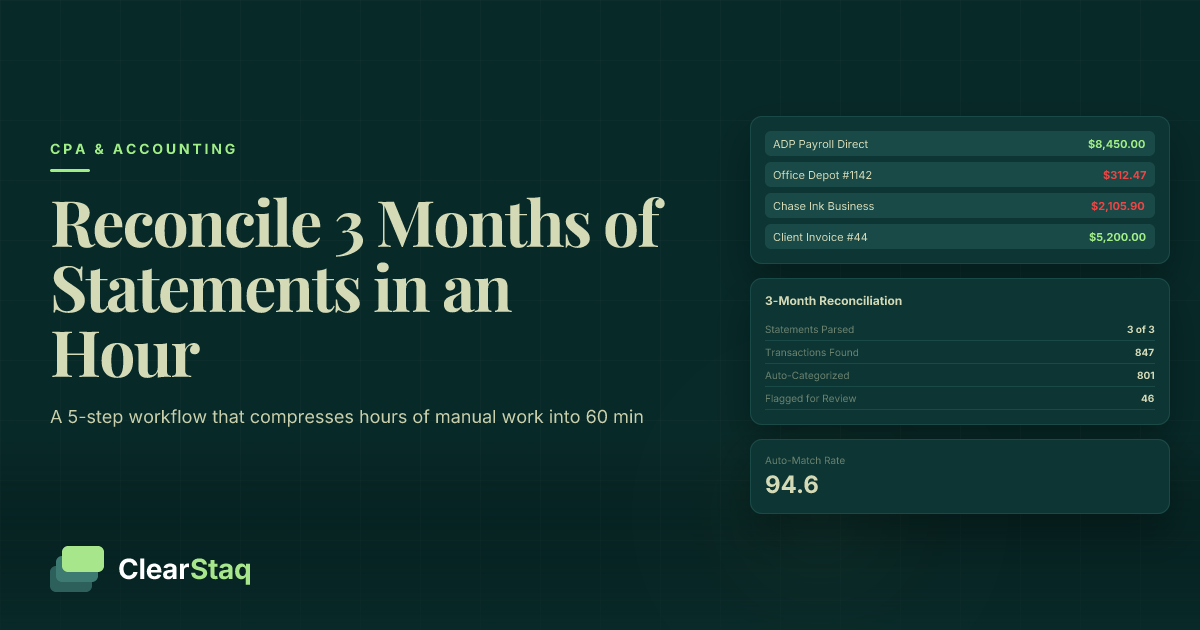
The foundation for any seasonality work is solid data — and that means starting with reconciling bank statements for a new client before building any seasonal baseline. Reconciliation isn't just about accuracy; it's about flagging intercompany transfers, duplicate entries, and non-operating deposits that would distort your seasonal curve from the start.

Normalizing for COVID-Era and Other Macro Distortions

2020 and 2021 data is problematic for nearly every industry. If your 24-month window includes those years, you need to make explicit normalization decisions before building any baseline. The BLS seasonal adjustment methodology provides a rigorous framework for treating exogenous shocks — the same logic applies here.

Identify and exclude one-time deposits that were common in those years: PPP loan deposits, EIDL grants, insurance payouts, and disaster relief payments. These inflated the deposit side of many businesses' statements in ways that have no recurring analog. Excluding them isn't optional if you want a defensible baseline.

Document every normalization decision in your working file. When a client questions why their 2021 peak doesn't show up in the benchmark, you need a clear, written rationale. That documentation also protects you if advisory recommendations are later questioned.

Step 1: Extract the Right Metrics from Bank Statements

The starting point for cash flow seasonality analysis is raw bank statement data — not exported accounting software data. Here's why that distinction matters: accounting software data has already been categorized, combined, and potentially adjusted. Bank statements show what actually moved in and out of the account, transaction by transaction, in the order it happened. That granularity is what makes seasonal pattern detection possible.

For each month, extract these core metrics:

• Total deposits — all funds received into the account
• Total withdrawals — all funds leaving the account
• Net cash flow — deposits minus withdrawals
• Average daily balance (ADB) — a liquidity indicator that smooths intra-month volatility
• Transaction count — a proxy for business activity volume
• NSF/overdraft events — a direct signal of cash stress in that month

Secondary metrics worth capturing include the largest single deposit in each month (flags one-time events), payroll frequency and amount (your fixed cost anchor), and recurring vendor payment totals.

Building Your Extraction Template

Structure your spreadsheet with one row per month and the following columns:

Month	Total Deposits	Total Withdrawals	Net Cash Flow	Avg Daily Balance	Transaction Count	NSF Events	Notes / Flags
Jan 2023	$42,100	$51,200	-$9,100	$8,400	87	2	Post-holiday trough
Feb 2023	$39,800	$48,600	-$8,800	$6,200	79	3	Trough continues
Nov 2023	$89,400	$54,100	+$35,300	$31,500	204	0	Holiday peak
Dec 2023	$101,200	$58,300	+$42,900	$44,700	231	0	Peak month

Create one sheet per account and one summary tab for the aggregated view. Flag any month where a non-recurring deposit distorts the total — keep both the raw figure and an adjusted figure in adjacent columns. Consistent column structure is what makes the seasonal curve visualization in Step 3 possible without reformatting.

Handling Clients with Multiple Bank Accounts

Clients with separate operating, payroll, and tax reserve accounts require aggregation before any seasonality analysis begins. The critical step is identifying intercompany transfers — funds moving from the operating account to the payroll account show up as a withdrawal in one statement and a deposit in another. Counting both inflates both totals and produces a meaningless seasonal curve.

Building a unified cash flow view across multiple accounts requires a consolidation step where intercompany transfers are netted out before monthly totals are calculated. This is where most CPA firms give up on seasonality analysis at scale — manual aggregation across three or more accounts from different banks in different PDF formats is genuinely time-intensive.

Step 2: Build Your Month-Over-Month Baseline

Once you have 12 to 24 months of extracted data in your template, the baseline is built in two stages: calculating monthly averages and smoothing them with a rolling trendline.

Start by calculating the average deposit total for each calendar month across all available years. If you have January 2022, January 2023, and January 2024, average those three figures to get your January baseline. Do this for all 12 months. The result is a 12-point seasonal profile — your benchmark curve.

Next, calculate the seasonal index for each month: divide that month's average by the overall annual monthly average (total annual deposits divided by 12). A December index of 1.55 means December deposits run 55% above the monthly average. A February index of 0.72 means February runs 28% below. Values above 1.0 are peak months; below 1.0 are trough months.

The Rolling 12-Month Average Explained

The rolling 12-month average is a smoothed trendline that sits underneath the seasonal curve and reveals the underlying business trajectory. At any given month, sum the prior 12 months of deposits and divide by 12. Plot that value alongside the monthly actual.

The separation between these two lines is where the real analytical insight lives. The monthly actuals show the seasonal pattern — the peaks and troughs. The rolling average shows whether the business is growing, flat, or declining beneath that pattern. A rising rolling average with consistent seasonal peaks is a healthy business. A declining rolling average — even if peak months still look strong in absolute terms — is an early warning signal that warrants discussion.

When the rolling average is falling even during peak months, that's not seasonal behavior. That's a trend problem wearing seasonal clothing.

Percentage Change vs. Seasonal Index: When to Use Each

Both metrics serve the cash flow benchmarking analysis, but they answer different questions.

Year-over-year (YoY) percentage change compares this November to last November. It's best for detecting whether the client's seasonal pattern is strengthening or weakening over time. A client whose November deposits grew 12% YoY while the industry average grew 8% is outperforming peers during the peak window — a positive advisory finding.

Seasonal index compares each month to the client's own annual average. It's best for identifying which months are structurally high or low, and for benchmarking one client's curve against another in the same industry. The index normalizes for business size, making peer comparisons meaningful even when absolute revenue levels differ significantly.

Use the index for benchmarking. Use YoY change for trend detection. Both belong in a complete seasonality analysis.

Step 3: Identify the Seasonal Curve (Peak, Trough, and Transition Months)

With your seasonal index calculated, label each month using a three-category framework:

• Peak: Seasonal index above 1.15 (more than 15% above the monthly average)
• Shoulder / Transition: Seasonal index between 0.85 and 1.15
• Trough: Seasonal index below 0.85 (more than 15% below the monthly average)

These thresholds are adjustable. A highly volatile seasonal business — agriculture, ski resorts — may warrant tighter thresholds. A business with modest seasonality may not cross 1.15 at all, in which case the distinction between high-shoulder and low-shoulder months becomes the relevant analysis.

The trough duration is one of the most practically important findings. A two-month trough is manageable with a modest cash reserve. A four-month trough — common in northern-climate construction — requires a materially different financing and reserve strategy. The seasonal map quantifies that difference in dollars.

Pay particular attention to transition months. These are the highest-risk period in any seasonal business: cash is declining as the trough approaches, but operating expenses haven't been reduced yet. NSF events and overdrafts cluster here, not in the deepest trough month, because that's when the cash buffer runs out. Identifying these months on the map gives you a specific intervention point to recommend to clients.

For more on how seasonal revenue patterns in bank statements surface across different business types, that resource covers the interpretation layer in additional depth.

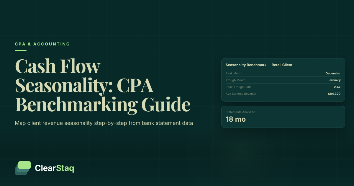
Industry Benchmark Curves: What Normal Looks Like

Comparing a client's curve to an industry benchmark is what separates a competent analysis from an exceptional one. Here are reference curves for the four most seasonally pronounced industries:

Industry	Peak Months	Peak Index Range	Trough Months	Trough Index Range
Retail	Nov–Dec	1.4–1.8x	Jan–Feb	0.60–0.75x
Restaurants (casual)	Jun–Aug	1.2–1.3x	Jan–Feb	0.70–0.80x
Construction (northern)	May–Sep	1.3–1.5x	Dec–Feb	0.50–0.70x
Agriculture	Oct–Nov	1.8–2.2x	Apr–Jun	0.40–0.60x

When a client's curve deviates significantly from these benchmarks — say, a retail client whose December index is only 1.1x — that deviation is the advisory finding, not the curve itself. A weaker-than-expected peak warrants a conversation about pricing, market positioning, or competitive dynamics before any cash flow recommendation is made.

Charting the Curve for Client Presentations

Non-financial clients process charts faster than tables. A 12-column bar chart — months on the X-axis, deposit totals or seasonal index on the Y-axis — with green bars for Peak months, yellow for Shoulder, and red for Trough is immediately readable by any business owner. You don't need to explain the methodology; the colors do the work.

Overlay the rolling 12-month average as a line on the same chart. Now the client can see both their seasonal pattern and their underlying trend in one view. Add a second chart with the prior year's curve for direct comparison, and you have a complete, presentation-ready deliverable that most clients have never seen before.

Step 4: Normalize for One-Time Events and Anomalies

A seasonal baseline is only useful if it reflects recurring operating behavior. One-time events distort both sides of the equation — deposits and withdrawals — and an unnormalized baseline produces wrong advisory conclusions.

On the deposit side, common one-time inflators include: PPP loans, EIDL grants, insurance payouts, equipment sale proceeds, tax refunds, and investor capital contributions. None of these represent recurring revenue. Including them in the baseline overstates the seasonal peak and makes ordinary operating months look like underperformance.

On the withdrawal side, watch for: legal settlements, major equipment purchases, one-time lease buyouts, and large tax payments. These inflate the withdrawal side in the month they occur and understate net cash flow for that period.

The normalization rule is simple: if a transaction wouldn't repeat under normal operating conditions, exclude it from the seasonal baseline — but document it clearly in the working file, not just the adjusted column.

How to Flag and Document Anomalies

Add a "Notes/Flags" column to your extraction template for every month where a non-recurring event occurred. Calculate an adjusted deposit total that removes the one-time item, and preserve both the raw and adjusted figures in adjacent columns.

When presenting to clients, show both curves side by side: the raw curve and the normalized curve. That comparison demonstrates the advisory value of the normalization step — clients can see exactly why one month looks different from what their bank statement total suggested. It also makes the methodology transparent, which builds trust.

Document the rationale for every exclusion. "PPP deposit of $87,400 received 4/15/2020 — excluded from operating baseline per normalization policy" is the kind of note that protects your work if a client later questions why their 2020 spring numbers look different from what they remember.

When Anomalies Are a Signal, Not Just Noise

Not every unusual deposit is noise. Large deposits that the client cannot explain clearly — especially if they recur in the same month across multiple years — warrant investigation before exclusion. Annual contract renewals, recurring insurance reimbursements, and annual royalty payments are legitimate operating revenue that may look like anomalies until you understand the business model.

NSF events clustered in trough months are not anomalies at all. They are the seasonal stress pattern manifesting, and they belong in the baseline analysis as a direct measure of how severe the trough is for that client. Normalizing them away would hide the finding you're trying to surface.

ClearStaq's parsing layer surfaces fraud signals and anomalous transaction patterns simultaneously with the extraction step — so the CPA conducting a seasonality review doesn't need a separate pass to flag potentially distorting deposits.

Step 5: Benchmark Against Industry Norms

Building a client's seasonal curve in isolation tells you what happened. Benchmarking it against industry norms tells you whether what happened is typical, exceptional, or a problem.

The benchmark questions that matter most for advisory CPAs are:

• Is the client's peak stronger or weaker than the industry average?
• Is the trough deeper or shallower than peers?
• Is the recovery from trough faster or slower than the industry curve suggests?

A client with a weaker-than-average peak is failing to capture revenue during the best window of the year — a strategic finding with real implications for pricing, marketing spend, and capacity management. A client with a deeper-than-average trough may have a fixed cost structure that's too high relative to their seasonal revenue — a cost structure advisory opportunity.

Data sources for industry benchmarks include SBA cash flow management guidance, BLS Business Employment Dynamics data, NAICS-level revenue seasonality indices, and your own firm's client portfolio data.

Building Your Own Benchmarks from Client Data

CPA firms with multiple clients in the same industry can build proprietary benchmarks from aggregated, anonymized client seasonal curves. Even five to ten clients in the same NAICS code produces a meaningful peer comparison — and that proprietary benchmark becomes a differentiating advisory asset that no bookkeeper or tax preparer can replicate.

When presenting peer comparisons, aggregate the benchmark data so no individual client is identifiable. "Based on our data from similar businesses in this industry" is sufficient framing. The client doesn't need to know the comparison pool — they need to know where they stand relative to it.

How to Tell the Difference Between Seasonality and Decline

This is the most consequential analytical judgment in the entire workflow. A misread here leads directly to wrong advisory recommendations — recommending a larger credit line for a "seasonal gap" that is actually structural revenue decline, for example, makes the problem worse, not better.

True seasonality looks like this: trough months are consistently low across multiple years, the rolling 12-month average is flat or growing, and peak months recover to prior-year levels or higher. The pattern repeats. The amplitude may vary slightly, but the shape is recognizable year over year.

Business decline masquerading as seasonality looks different: trough months get progressively deeper each cycle, the rolling 12-month average trends downward, and — critically — peak months fail to recover to prior-year levels. The seasonal shape may still be present, but the entire curve is shifting downward.

The dual test: (1) Is this year's trough lower than last year's trough? (2) Is this year's peak lower than last year's peak? If both answers are yes, decline is more likely than pure seasonality. The second question — peak performance — is the more reliable signal. Seasonal businesses have volatile troughs; what they don't have is declining peaks.

For the perspective lenders apply to the same analytical challenge, seasonality analysis in bank statements from an MCA underwriting context covers how this distinction is made in credit decisioning — useful context for CPAs advising clients on financing options.

Warning Signs Hidden in the Seasonal Pattern

These specific signals suggest decline rather than normal cash flow seasonality analysis:

• Trough depth increasing year over year — this January is materially worse than last January
• Recovery from trough taking longer each cycle — March used to be a Shoulder month; now it's still in Trough territory
• Peak months plateauing or declining even when industry-wide seasonal strength is present
• NSF and overdraft events appearing earlier in the trough cycle than in prior years — a sign the cash buffer is eroding

How to Present a Decline Finding to a Client

Lead with the data, not the diagnosis. Show the year-over-year chart before stating any conclusion. The visual does more work than any verbal explanation, and it keeps the conversation factual rather than emotional.

Frame findings as observations that invite discussion: "Your January deposits have declined 18% compared to the same month two years ago — is there a strategic reason for that?" The AICPA advisory communication framework consistently recommends this approach: findings open a conversation, they don't deliver a verdict.

Also be clear about the limits of bank statement data. Revenue decline visible in deposits may or may not reflect margin changes — and the bank statement alone won't tell you which. That distinction may require a deeper financial review before you can make a confident advisory recommendation.

Turning the Seasonal Map into Client Advisory Recommendations

The seasonal map is not the deliverable. It's the input. The actual value a CPA delivers sits in the recommendations that follow from the map — and those recommendations fall into three domains: financing timing, cash reserve strategy, and operational planning.

Financing timing is the most immediately actionable recommendation for most seasonal clients. The guidance is counterintuitive but important: draw on lines of credit 60 to 90 days before the trough begins, not during the trough when lender risk perception is highest and cash flows look worst on paper. A seasonal map gives you the specific month to cite: "Based on your pattern, you should have your line of credit drawn by mid-September before the November-February contraction begins."

Cash reserve strategy requires quantifying the trough funding gap — the total cumulative net cash flow deficit across all trough months. That figure becomes the basis for a specific reserve recommendation. "You need approximately $X in available cash or credit before your trough begins" is a more useful advisory output than "build a cash cushion."

Operational planning maps naturally to the seasonal curve as well. Trough months are the right window for negotiating vendor payment extensions, deferring non-essential capital expenditures, and running off-season promotions. The map tells you exactly when those conversations need to happen — not generically, but for this client, in this geography, in this industry.

Calculating the Trough Funding Gap

The formula is straightforward: sum the monthly net cash flow (deposits minus withdrawals) across all trough months. That total is the baseline funding gap. Add a 15 to 20% buffer for unexpected expenses — equipment failure, an unexpected tax payment, a slow-paying customer — and you have a defensible credit facility recommendation.

Sensitivity analysis adds advisory credibility. Show the client what happens to the funding gap if their trough deepens by 10% compared to last year. That scenario is concrete and visible, not hypothetical. Clients who see their own data used in a downside scenario understand the stakes of the recommendation in a way that abstract advice never achieves.

How Seasonal Maps Feed Into Quarterly Business Reviews

Once a seasonal baseline exists, every quarterly business review has a ready-made structure. The first question in any QBR becomes: "How did this quarter's actual performance compare to your seasonal expectation?" A variance from the baseline — positive or negative — is the starting point for the conversation, not trailing financials reviewed in isolation.

When it comes to automating quarterly business reviews, the seasonal benchmark is the anchor that makes each review more structured and insight-driven. Clients who receive seasonal benchmarking as part of their QBR package consistently perceive higher advisory value — with measurable retention and upsell impact for the firms that deliver it.

How Automated Bank Statement Parsing Speeds Up the Process

The methodology described in this guide is analytically sound. The barrier to deploying it at scale is the data extraction step, not the analysis. Pulling month-by-month deposit totals, average daily balances, and transaction counts from PDF bank statements for 24 months across multiple accounts takes four to eight hours per client manually. That's why most CPA firms don't offer cash flow seasonality analysis as a standard service — not because they lack the expertise, but because the data gather makes it economically impractical at volume.

Automated bank statement parsing eliminates that bottleneck entirely. Structured data — monthly totals, average daily balance, transaction counts, NSF flags — is returned in minutes, not hours. There's no manual data entry between the PDF and the spreadsheet template.

For firms looking to automate bank statement processing, the efficiency case is straightforward: the same analysis that takes half a day per client manually takes minutes with parsed, structured output. That time difference is the difference between seasonality mapping as a boutique offering for top-tier clients and seasonality mapping as a standard service across an entire advisory portfolio.

ClearStaq supports 900+ bank formats, which means consistent structured output regardless of whether the client banks at Chase, a regional credit union, or a community bank in a format you've never seen before. Multi-account aggregation — combining statements from multiple banks and accounts into a unified month-over-month view — happens before the CPA opens the spreadsheet, with intercompany transfers identified and flagged in the output. ClearStaq's CPA advisory tools are built specifically for this workflow.

Fraud signals surface simultaneously. During a seasonality review, anomalous deposits that could distort the baseline are flagged automatically — the CPA doesn't need a separate fraud review pass. One workflow, two outputs: the seasonal data and the anomaly flags.

What the Automated Extraction Workflow Looks Like

The process is four steps:

1. Upload client bank statement PDFs — any format, any bank
2. Receive structured JSON or CSV output with month-by-month deposit totals, withdrawals, average daily balance, and transaction counts
3. Import into the seasonality mapping spreadsheet template — no manual data entry required
4. Begin analysis immediately — the data gather that used to take half a day is complete in minutes

From Parsing Output to Seasonal Map in One Workflow

ClearStaq's API feeds structured data directly into spreadsheet templates or client reporting dashboards. A 24-month trend dataset is surfaced in a single API response for multi-month statement batches — no need to run multiple queries or stitch together separate outputs.

For firms processing multiple clients, batch processing means an entire advisory portfolio's seasonal maps can be updated monthly without incremental labor. The scalability argument is real: a firm that automates extraction can offer seasonality mapping to ten times more clients without adding staff. That's not an efficiency gain — it's a practice transformation.

Frequently Asked Questions

What is revenue seasonality mapping?

Revenue seasonality mapping is the process of analyzing 12 to 24 months of a business's bank statement data to identify recurring cash flow peaks, troughs, and transition months. CPAs use it to build a month-over-month benchmark that informs advisory recommendations on cash reserves, financing timing, and operational planning.

How many months of bank statements do you need to identify seasonality?

A minimum of 12 months is required to complete one seasonal cycle, but 24 months is the preferred dataset because it allows year-over-year comparison and helps distinguish a true repeating pattern from a one-year anomaly. For clients with COVID-era distortions in 2020 to 2021, 36 months of data is ideal to establish a reliable baseline.

How do CPAs analyze cash flow seasonality for clients?

CPAs extract monthly deposit totals, average daily balances, and transaction counts from raw bank statements, then calculate each month's deviation from the annual average to produce a seasonal index. Months are labeled as Peak, Shoulder, or Trough, and the resulting curve is benchmarked against industry norms to identify whether the client's pattern is typical or an outlier requiring advisory action.

How do you tell the difference between seasonal dips and business decline?

The key test is comparing year-over-year peak performance: a seasonal business has stable or growing peak months even when trough months are low. If peak months are also declining year over year alongside deepening troughs, and the rolling 12-month average is falling, that pattern indicates business decline rather than normal cash flow seasonality analysis.

What tools do CPAs use to analyze client cash flow seasonality?

Most CPAs still rely on spreadsheets built manually from exported accounting software data or PDF bank statements. Automated bank statement parsing tools like ClearStaq extract month-by-month deposit totals, average daily balances, and transaction counts directly from raw PDFs across 900+ bank formats, eliminating the manual data entry step that makes seasonality mapping time-prohibitive at scale.

How do you benchmark monthly cash flow for a small business client?

Calculate a seasonal index by dividing each month's average deposit total by the overall annual monthly average across 24 months of data. Values above 1.0 identify peak months; values below 1.0 identify trough months. Compare that index against industry benchmarks — using BLS, SBA, or your own firm's client portfolio data — to determine whether the client is outperforming, underperforming, or aligned with peers in the same NAICS code.